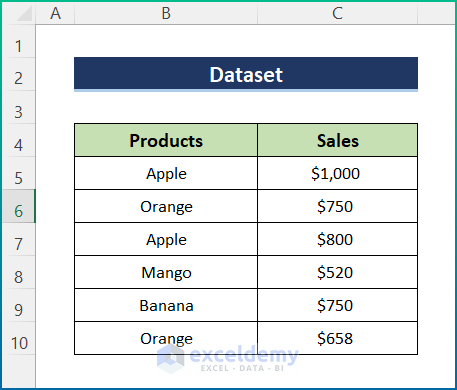
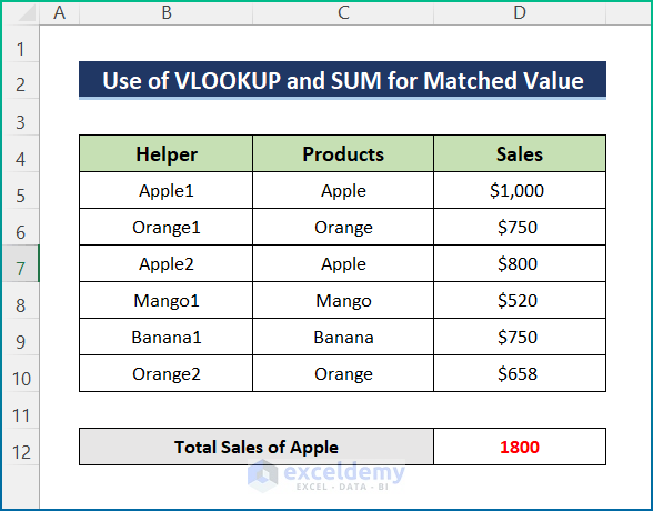
In the dataset below, we have two columns displaying Products and Sales.
Method 1 – Using VLOOKUP and Sum Matched Values in Multiple Rows
Steps:
- Enter the following formula in cell B5 to create the Helper Column.
=C5&COUNTIF($C$5:$C5,C5)
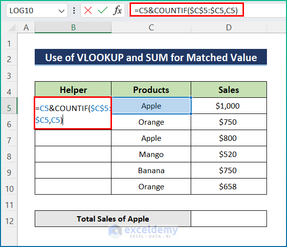
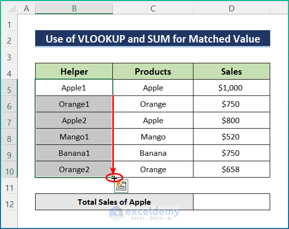
- Click Enter and use the AutoFill tool to the whole column.
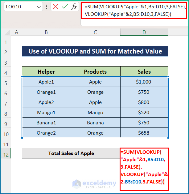
- Select cell D12 and enter the following formula:
=SUM(VLOOKUP("Apple"&1,B5:D10,3,FALSE),VLOOKUP("Apple"&2,B5:D10,3,FALSE))
Formula Breakdown:
- The VLOOKUP function matches the criteria Apple with ranges B5:D10 from the dataset.
- Here, you have to search twice, as the Helper column shows Apple twice.
- The VLOOKUP function extracts the values of the matched cells.
- The SUM function provides the sum of the output values provided by the VLOOKUP function.
- Hit Enter to get the total sales of Apples.
Read More: How to Use VLOOKUP for Rows in Excel
Method 2 – Inserting the SUMPRODUCT Function to VLOOKUP and Sum
Steps:
- Select cell C12 and enter the following formula:
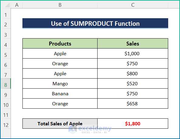
=SUMPRODUCT((B5:B10="Apple")*C5:C10)
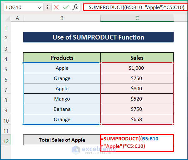
- Press Enter to get a similar output.
Read More: How to VLOOKUP and SUM Across Multiple Sheets in Excel
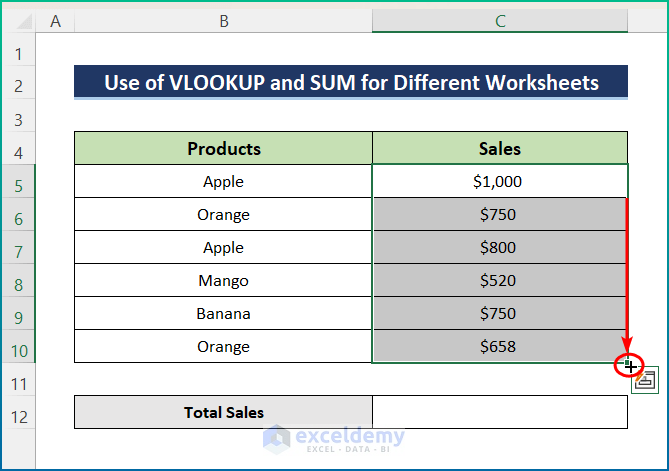
Method 3 – Using VLOOKUP and Sum Multiple Rows from Different Worksheets
Steps:
- Click on cell C5 and enter the formula below:
=VLOOKUP(B5, Dataset!B5:C10, {2}, FALSE)
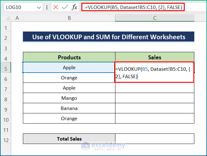
Note: In the formula, {2} indicates the column index number. It starts from 1, which indicates the first column in an Excel sheet. Here, our dataset starts from the second column, so we used 2 as the column index.
- Apply the AutoFill tool to the entire column of the dataset.
- Select cell C12.
- Enter the following formula:
=SUM(C5:C10)
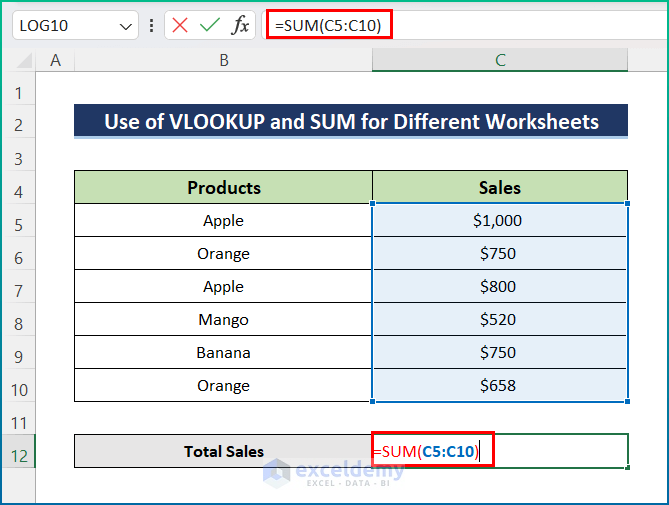
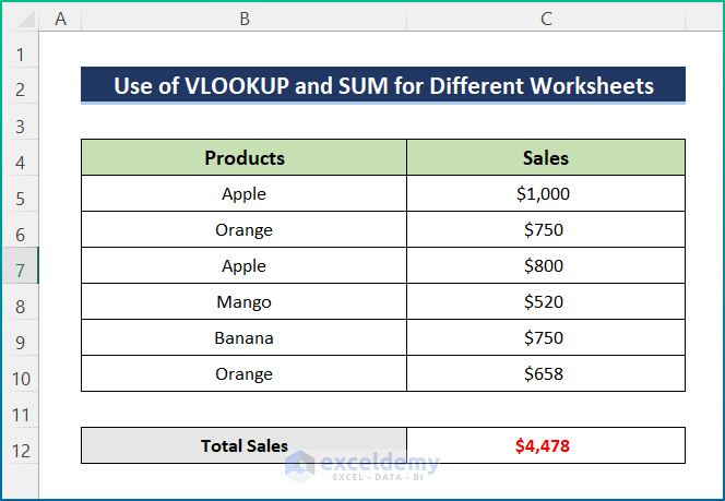
- Press the Enter button to get the result.
Read More: How to Combine SUMIF and VLOOKUP in Excel
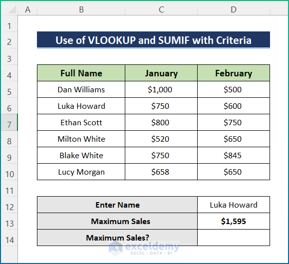
Method 4 – Using VLOOKUP and SUMIF Multiple Rows with Criteria
Steps:
- Select cell D13 and enter the formula below:
=MAX(SUM(C5:D5),SUM(C6:D6),SUM(C7:D7),SUM(C8:D8),SUM(C9:D9),SUM(C10:D10))
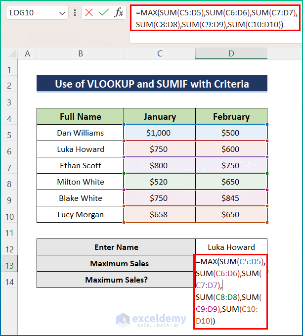
- Press the Enter button to find the Maximum Sales.
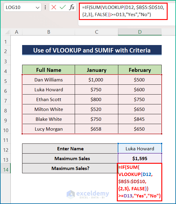
- Enter the formula below in cell D14:
=IF(SUM(VLOOKUP(D12, $B$5:$D$10,{2,3}, FALSE))>=D13,"Yes","No")
Formula Breakdown
- In the IF function, SUM(VLOOKUP(D12, $B$5:$D$10, {2,3}, FALSE))>=D13 is the logical condition.
- {2,3} is an argument of the VLOOKUP function, which indicates the column index number. Usually, it starts from 1, which indicates the first column in an Excel sheet.
- However, the VLOOKUP function checks if the entered Name’s total sales are greater than or equal to our predefined maximum sales or not. Here, it searched for Luka Howard and provided the amount of sales for January and February.
- The SUM function provides the sum of the sales amount received from the VLOOKUP function. However, the output is 1350$.
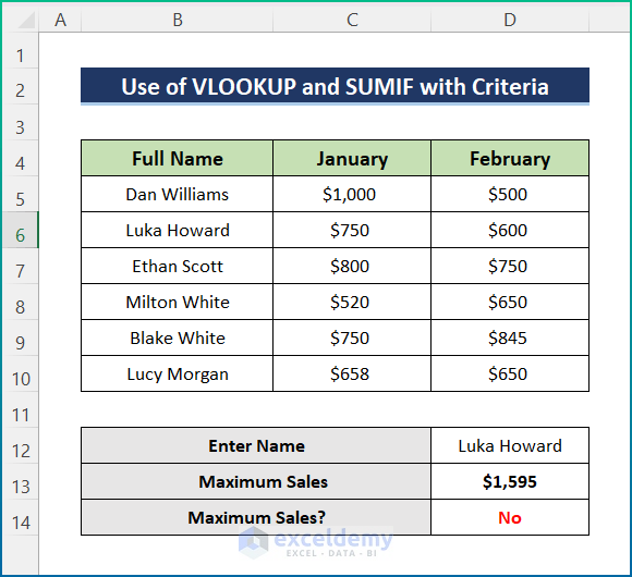
- The IF function checks the condition. Here, the maximum sale is given as 1595$, and the formula will check whether the output we received is maximum or not. If the sales match, it will print “Yes”; otherwise, “No.”
- Hit the Enter key to get the final result.
Read More: INDEX MATCH vs VLOOKUP Function
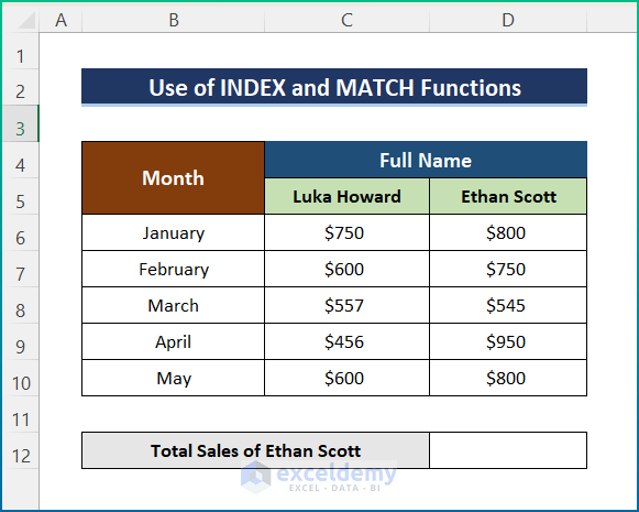
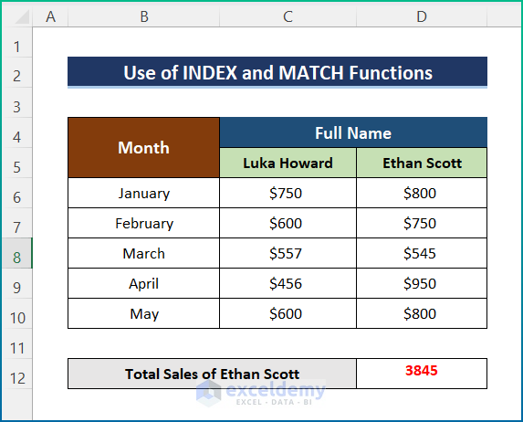
How to Sum Multiple Rows with INDEX and MATCH Functions
Here, we will calculate the total sales of employee Ethan Scott for various months of the year. For the purpose of demonstration, the dataset has been changed.
Steps:
- Enter the following formula in cell D12:
=SUM(INDEX(C5:D10,,MATCH("Ethan Scott",C5:D5,0)))
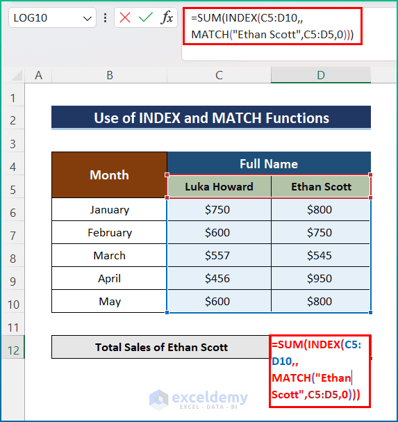
- Press Enter to calculate the total sales of Ethan Scott.
Things to Remember
- If the searched value is absent in the given dataset, all these functions will return this #NA Error.
- If col_index_num is greater than the number of columns in the table array, you’ll get the #REF! Error value.
- You’ll get the #VALUE! Error value If the table_array is less than 1.
Download the Practice Workbook
You can download the workbook used for the demonstration from the download link below.
Further Readings
- Combining SUMPRODUCT and VLOOKUP Functions in Excel
- How to Use VLOOKUP with COUNTIF
- Excel LOOKUP vs VLOOKUP
- XLOOKUP vs VLOOKUP in Excel
- How to Use Nested VLOOKUP in Excel
- IF and VLOOKUP Nested Function in Excel
- How to Use IF ISNA Function with VLOOKUP in Excel
- How to Use IFERROR with VLOOKUP in Excel
- VLOOKUP with IF Condition in Excel
<< Go Back to Excel VLOOKUP Sum | Excel VLOOKUP Function | Excel Functions | Learn Excel
Get FREE Advanced Excel Exercises with Solutions!

JazzakAllahKhair Brother.
Hey, man. It looks like you are getting the sum of the columns (not the rows as indicated) in the first example.
what {2,3} mean?
Hello QUAN,
Thanks for your question. Here, {2,3} defines the cell number of the defined range B5:D10. 2 defines the row number and 3 defines the column number. Setting B5 as the base point and moving two rows and three columns, we will have the D6 cell which is expressed here with {2,3}.