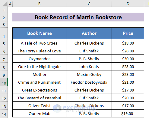
Consider the following dataset which contains a bookstore’s stock. We’ll use the VLOOKUP function to sum all matches for a particular criteria.
3 Easy Ways to Sum All Matches with VLOOKUP in Excel
We’ve got a data set with the Names, Authors, and Prices of some books from a bookshop.
Method 1 – Use the FILTER Function to Sum All Matches with VLOOKUP in Excel 365
- Enter the following formula to find the sum of the prices of all the books by Charles Dickens:
=SUM(FILTER(D5:D14,C5:C14=F5))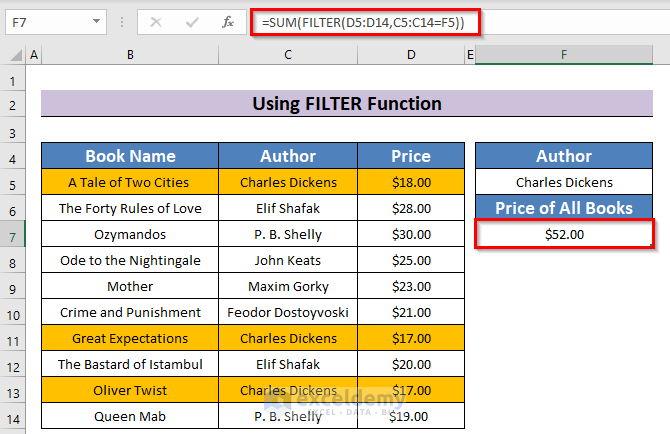
⧪ Explanation of the Formula:
- The FILTER function matches a lookup value with all the values of a lookup column and returns the corresponding values from another column.
- F5 (Charles Dickens) is our lookup value, C5:C14 (Author) is the lookup column, and D4:D13 (Price) is the other column.
- FILTER(D4:D13,C5:C14=F4) matches all values of the column C5:C14 (Author) with F5 (Charles Dickens) and returns the corresponding values from the column D4:D13 (Price).
- SUM(FILTER(D4:D13,C5:C14=F5)) returns the sum of all the prices of all the books returned by the FILTER function.
- You can change the lookup value to any other author except Charles Dickens in cell F5, and it will return the total price of the books of that author.
Read More: How to Vlookup and Pull the Last Match in Excel
Method 2 – Use the IF Function to Sum All Matches with VLOOKUP in Excel (For Older Versions of Excel)
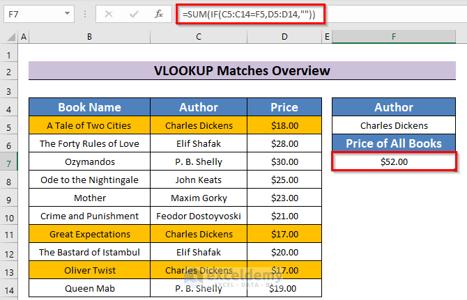
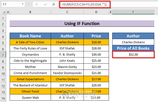
- The sum of the prices of all the books of Charles Dickens can be found using this formula:
=SUM(IF(C5:C14=F5,D5:D14,""))[This is an Array Formula. Press Ctrl + Shift + Enter to apply it unless you use Office 365.]
⧪ Explanation of the Formula:
- IF(C5:C14=F5,D5:D14,””) matches all values of the lookup column C5:C14 (Author) with the lookup value F5 (Charles Dickens).
- If the lookup value F5 matches the lookup column C5:C14 (Author), then it returns the corresponding value from the column D5:D14 (Price). If it doesn’t match, it returns a blank string “”.
- SUM(IF(C5:C14=F5,D5:D14,””)) returns the sum of all the values returned by the IF function.
Read More: How to Vlookup and Sum Across Multiple Sheets in Excel
Method 3 – Use the VLOOKUP Function to Sum All Matches with VLOOKUP in Excel (For Older Versions of Excel)
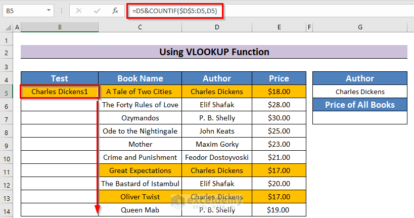
- Select the column left to the data set and enter this formula in the first cell (B5).
=D5&COUNTIF($D$5:D5,D5)
Note: D5 is the first cell of the lookup array (Author). You use the one from your data set.
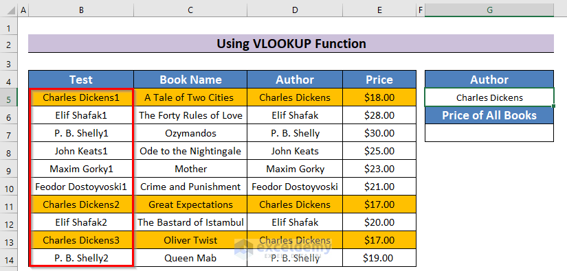
- Drag the Fill Handle down to fill the column.
- This will create a sequence of the authors along with the ranks (repetitions in the array), such as Charles Dickens1, Charles Dickens2, Elif Shafak1, Elif Shafak2 and so on.
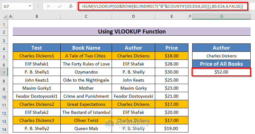
- Enter the lookup value in a new cell. We have entered Charles Dickens in cell G5.
- Enter the following formula in the result cell:
=SUM(VLOOKUP(G5&ROW(B1:INDIRECT("B"&COUNTIF(D5:D14,G5))),B5:E14,4,FALSE))[This is an Array Formula. Press Ctrl + Shift + Enter to apply it unless you’re using Office 365.]
⧪ Explanation of the Formula:
- COUNTIF(D5:D14,G5) returns 3, as there are a total of 3 cells in the range D5:D14 (Author) that contain the lookup value G5 (Charles Dickens). See the COUNTIF function for details.
- B1:INDIRECT(“B”&COUNTIF(D5:D14,G5)) now becomes B1:B3. See the INDIRECT function for details.
- G5&ROW(B1:INDIRECT(“B”&COUNTIF(D5:D14,G5))) becomes G5&{1, 2, 3} and returns an array {Charles Dickens1, Charles Dickens2, Charles Dickens3}.
- VLOOKUP(G5&ROW(B1:INDIRECT(“B”&COUNTIF(D5:D14,G5))),B5:E14,4,FALSE) now becomes VLOOKUP({Charles Dickens1, Charles Dickens2, Charles Dickens3},B5:E14,4,FALSE).
- The VLOOKUP function matches the lookup value with all the values of the first column of the data set and then returns the corresponding values from another column.
- Here the lookup value is the array {Charles Dickens1, Charles Dickens2, Charles Dickens3}.
- Therefore, it matches the lookup values with all the values of the first column B5:E14, and returns the corresponding values from the 4th column (Price).
- The SUM function returns the sum of all the prices that match the lookup values.
Read More: How to Use VLOOKUP with SUM Function in Excel
Download the Practice Workbook
Related Articles
- Excel VBA to Match Value in Range
- How to Match Names in Excel Where Spelling Differ
- Excel VBA: Copy Row If Cell Value Matches
- How to Return Row Number of a Cell Match in Excel
- How to Sum Top n Values in Excel
<< Go Back to Excel VLOOKUP Sum | Excel VLOOKUP Function | Excel Functions | Learn Excel
Get FREE Advanced Excel Exercises with Solutions!

Hello,
So I’m trying to create a sum of two separate columns with the vlook from two different columns equals a given name.
What I have is an excel spreadsheet that downloads from an external platform. The scenario is:
If column “K” is blank then I need the sum of column “N” for any rows with the label “asphalt field” in column “I” and if column “K” has a matching label then I need the sum of columns “j” & “L” that match the label?
I have been trying various different formula setups but this is way above my ability. please help!
Hi KEITH,
Your problem is partly vague I think. Still, I’ve tried to build a formula that might work for you. If this doesn’t work, I would recommend you share your workbook with me or at least share a sneak peek of your dataset.
Now use this formula:
=IF(ISBLANK(K2),SUMIF(I2:I13,”asphalt field”,N2:N13),SUM(J2:J13,L2:L13))
Thanks!
Thank you, this helped me
Hello LN,
You are most welcome. Thanks for your feedback and appreciation. Glad to heart that our article helped you.
Keep exploring Excel with ExcelDemy!
Regards
ExcelDemy