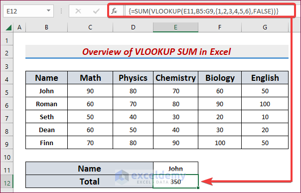
This article will show you how to use the VLOOKUP function with the SUM function to execute certain operations in Excel. Before diving into the methods, have a look at the overview image below.
VLOOKUP Function in Excel: Syntax
VLOOKUP stands for ‘Vertical Lookup‘. It searches for a certain value in a column and returns a value from a different column in the same row.
Generic Formula:
=VLOOKUP(lookup_value, table_array, col_index_num, [range_lookup])| Arguments | Definition |
|---|---|
| lookup_value | The value you are trying to match |
| table_array | The data range that you want to search your value |
| col_index_num | Corresponding column of the lookup_value |
| range_lookup | This is a Boolean value: TRUE or FALSE. FALSE (or 0) means exact match and TRUE (or 1) means approximate match. |
Method 1 – Calculating Matching Values in Columns Using VLOOKUP with the SUM Function in Excel
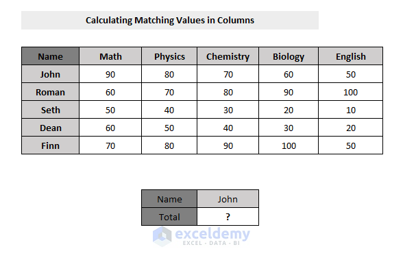
Consider the following dataset which consists of students’ names and their obtained marks on each course stored in different columns. What if you want to find out just a particular student’s total marks? To get that, you have to calculate numbers based on different columns.
Steps:
- Put the search term in a separate cell (e.g. John in Cell E12).
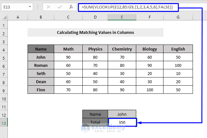
- Click on the cell where you want the result to appear (e.g. Cell E13).
- Insert the following formula:
=SUM(VLOOKUP(E12,B5:G9,{1,2,3,4,5,6},FALSE))E12 = John, the name that we stored as the lookup value
B5:G9 = Data range to search the lookup value
{1,2,3,4,5,6} = Corresponding columns of the lookup values (columns that has John’s marks on each course stored)
FALSE = As we want an exact match, so we put the argument as FALSE.
- Press Ctrl + Shift + Enter.
Formula Breakdown:
- VLOOKUP(E12,B5:G9,{1,2,3,4,5,6},FALSE) -> looking for E12 (John) in the B5:G9 (array) and returning the exact corresponding columns values ({1,2,3,4,5,6}, FALSE).
Output: 90,80,70,60,50 (which is exactly the marks John achieved on individual courses)
- SUM(VLOOKUP(E12,B5:G9,{1,2,3,4,5,6},FALSE)) -> becomes SUM(90,80,70,60,50)
Output: 350 (John’s total marks)
Method 2 – Determining Matching Values in Rows with Excel VLOOKUP and SUM Function
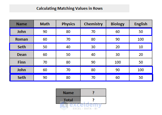
Consider the following dataset which consists of students’ names and their obtained marks on each course stored in different columns. However, students are allowed to retake exams, and their scores are put in a different row. What if you want to find out just those particular students’ total marks who have retaken the exam?
Steps:
- Insert a value in the cell for the search term (in our case, Cell E13).
- Click on another cell where you want the result to appear (e.g. Cell E14).
- Use the following formula:
=SUMPRODUCT((B5:B11=E13)*C5:G11)
Formula Breakdown:
- B5:B11=E13 -> looks for the match of the lookup value (e.g. John in Cell E13) throughout the array of Name column (B5:B11) and returns TRUE or FALSE based on the search.
Therefore, Output: {TRUE;FALSE;FALSE;FALSE;FALSE;TRUE;FALSE}
As we got TRUE values so now we know that there are matched values in the dataset. It is not a constant value-extracting process. Because we can write any name from the dataset in that cell (E13) and the result will be auto-generated in the result cell (e.g. E14). (see the picture above)
- SUMPRODUCT((B5:B11=E13)*C5:G11) -> becomes SUMPRODUCT{TRUE;FALSE;FALSE;FALSE;FALSE;TRUE;FALSE}*(C5:G11) which means, the SUMPRODUCT function then multiplies the TRUE/FALSE return value with the return array and produce the result of only for the TRUE values and pass it to the cell. FALSE values are actually canceling the unmatched data of the table array, leading to only the matched values appearing on the cell.
Output: 750 (John’s total marks with the retaken exam)
Method 3 – Generating Values in Two Different Worksheets by Using VLOOKUP with the SUM Function
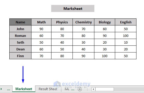
We have exam marks of students in the Excel worksheet named Marksheet.
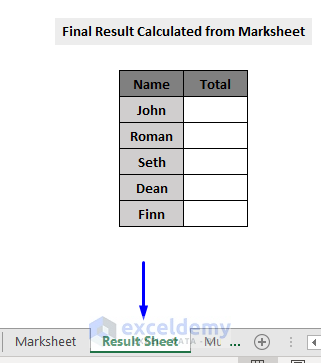
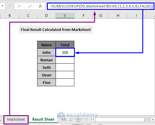
And in the worksheet named Result Sheet, we want to have all the students’ totals.
Steps:
- Select the cell for the first result.
- In that cell, use the following formula.
=SUM(VLOOKUP(D5,B5:G9,{1,2,3,4,5,6},FALSE)- Since this worksheet doesn’t have any data to be considered, it will produce an error. Place the pointer of your mouse before the array declaration in the formula (e.g. B5:G9), and select the other sheet that you want your values from.

- This will auto-generate a link to the sheet.
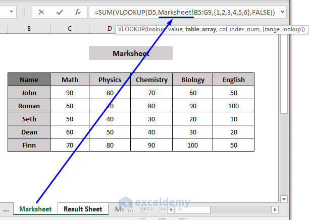
- The formula becomes:
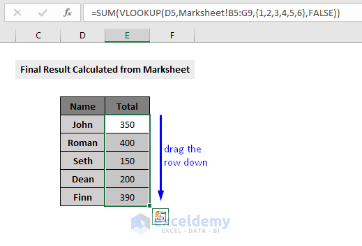
=SUM(VLOOKUP(D5,Marksheet!B5:G9,{1,2,3,4,5,6},FALSE))- Press Enter and you will get the desired result.
- Drag the row down via the Fill Handle to apply the formula to the rest of the rows to get the results.
Read more: How to Vlookup and Sum Across Multiple Sheets in Excel
Method 4 – Applying VLOOKUP and SUM Functions to Measure Values Across Multiple Worksheets
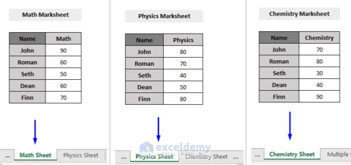
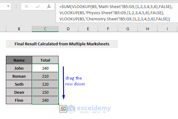
Consider the following data where we have three different worksheets named Math Sheet, Physics Sheet and Chemistry Sheet. Let’s get the totals from these sheets.
- The formula will look like this:
=SUM(VLOOKUP(B5,'Math Sheet'!B5:G9,{1,2,3,4,5,6},FALSE),VLOOKUP(B5,'Physics Sheet'!B5:G9,{1,2,3,4,5,6},FALSE),VLOOKUP(B5,'Chemistry Sheet'!B5:G9,{1,2,3,4,5,6},FALSE))- Press Enter and you will get the desired result.
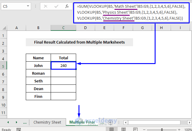
- Drag the row down via the Fill Handle to apply the formula to the rest of the rows to get the results.
Similar Readings:
- How to VLOOKUP with Multiple Conditions in Excel (2 Methods)
- Combine SUMIF and VLOOKUP Excel (3 Quick Approaches)
Method 5 – Combining VLOOKUP with the SUM Function in Excel to Sum up Values in Different Columns
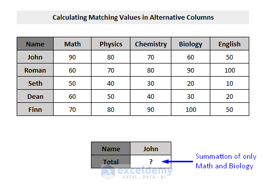
Consider the following dataset which consists of students’ names and their obtained marks on each course stored in different columns. What if you want to find out just a particular student’s total marks based on some specific courses? To get that, you have to calculate numbers based on alternative columns.
Steps:
- Insert the value you want to search in cell E12.
- Click on another cell where you want the result to appear (e.g. Cell E13).
- Use the following formula,
=SUM(VLOOKUP(E12,B5:G9,{2,5},FALSE))
- E12 = John, the name that we stored as the lookup value
- B5:G9 = Data range to search the lookup value
- {2,5} = Corresponding columns of the lookup values (columns that has John’s marks on only Math & Biology courses stored)
- FALSE = As we want an exact match, so we put the argument as FALSE.
- Press Ctrl + Shift + Enter on your keyboard.
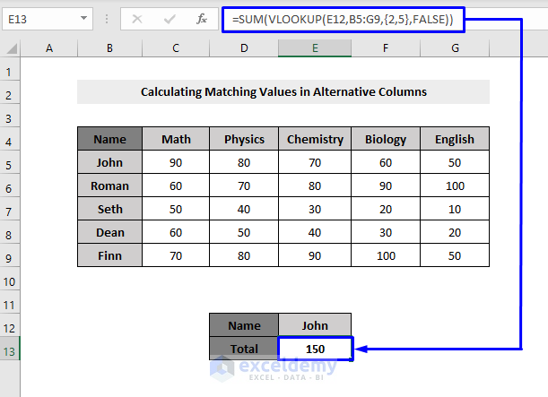
This process will give you the result of 150 (marks in Math and Biology).
Formula Breakdown:
- VLOOKUP(E12,B5:G9,{2,5},FALSE) -> looking for E12 (John) in the B5:G9 (array) and returning the exact corresponding columns values of Math and Biology ({2,5},FALSE).
So, Output: 90,60 (which is exactly the marks John achieved on Math and Biology)
- SUM(VLOOKUP(E12,B5:G9,{2,5},FALSE)) -> becomes SUM(90,60)
Output: 150 (John’s total marks on Math and Biology)
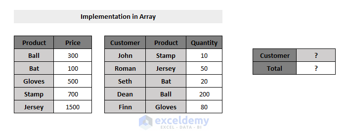
Method 6 – Using Excel VLOOKUP with the SUM Function in an Array
Look at the following dataset, where we need to find out not only just the name of the customer but also the total cost of the purchase.
Steps:
- Insert the search value in cell J5.
- Click on another cell where you want the result to appear (e.g. Cell J6).
- Use the following formula:
=SUM(VLOOKUP(F5:F9,B5:C9,2,FALSE)*G5:G9*(E5:E9=J5))
Formula Breakdown:
- VLOOKUP(F5:F9,B5:C9,2,FALSE) -> it looks for the exact name (FALSE argument) of all the Products (F5:F9) from the second table, in the Product array (B5:C9) from the first table and returns the price of that product (column index 2).
Therefore, Output: 700,1500,100,300,500
- VLOOKUP(F5:F9,B5:C9,2,FALSE)*G5:G9 -> G5:G9 refers to the Quantity column of the dataset.
So, VLOOKUP(F5:F9,B5:C9,2,FALSE)*G5:G9 becomes {(700,1500,100,300,500)*(10,50,20,200,80)}.
Output: 7000,75000,2000,60000,40000
- E5:E9=J5 -> it looks for the match of the lookup value (e.g. John in Cell J5) throughout the array of Name column (E5:E9) and returns TRUE or FALSE based on the search.
Lastly, Output: {TRUE;FALSE;FALSE;FALSE;FALSE}
Since we got TRUE values, we know that there are matched values in the dataset. It is not a constant value extracting process. Because we can write any name from the dataset in that cell (J5) and the result will be auto-generated in the result cell (e.g. J6).
- VLOOKUP(F5:F9,B5:C9,2,FALSE)*G5:G9*(E5:E9=J5) -> becomes (7000,75000,2000,60000,40000)*({TRUE;FALSE;FALSE;FALSE;FALSE}), it multiplies the TRUE/FALSE return value with the return array and produce the result only for the TRUE values and pass it to the cell. FALSE values are actually cancelling the unmatched data of the table array, leading to only the matched values appearing on the cell (J6), meaning, if you put the name John from the Name dataset (E5:E9) in the cell J5, it will only generate the total purchase (7000) of John, if you put name Roman, it will produce 75000 in the result cell (J6). (see the picture above)
Subsequently, Output: 7000,0,0,0,0
- SUM(VLOOKUP(F5:F9,B5:C9,2,FALSE)*G5:G9*(E5:E9=J5)) -> becomes SUM(7000)
Output: 7000 (which is exactly the total purchase amount of John)
Keep in Mind
- As the range of the data table array to search for the value is fixed, don’t forget to put the dollar ($) sign in front of the cell reference number of the array table.
- When working with array values, don’t forget to press Ctrl + Shift + Enter on your keyboard while extracting results. Pressing only Enter will work only when you are using Microsoft 365.
- After pressing Ctrl + Shift + Enter, you will notice that the formula bar encloses the formula in curly braces {}, declaring it as an array formula. Don’t type those brackets {} yourself, as Excel automatically does this for you.
Download the Practice Template
You May Also Like To Explore
- How to Make VLOOKUP Case Sensitive in Excel (4 Methods)
- Excel VLOOKUP to Find the Closest Match (with 5 Examples)
- How to Perform VLOOKUP with Wildcard in Excel (2 Methods)


I have a multi sheet spread sheet keeping track of job hours. I have used VLOOKUP in succession to sum all the hours on multiple sheets and it works great… Until it gets to a sheet that does not contain the lookup value. I have searched all over for my issue, and VLOOKUP may be the incorrect solution. I was wondering if I could rattle anyone’s brain to make this work.
I.E. I have 1 excel document with 52 tabs. Each tab is a work week starting from January so WW1 is all the hours FOR sed jobs I did for that week. “joes house 2 hours ; mikes house 3 hours”… WW2, WW3 etc… Until WW52.
This is the function I made to add hours together…
=SUM(VLOOKUP(O30,’WW29′!$A$7:$M$110,{13},FALSE),VLOOKUP(O30,’WW30′!$A$7:$M$110,{13},FALSE),VLOOKUP(O30,’WW31′!$A$7:$M$110,{13},FALSE)) And it works great. But when that job is finished it is not on (for example WW32 tab). Hence I get the #N/A error. so for example, as the previous one works great when I expand the formula to cover all 52 sheets… (EXAMPLE OF NEXT PAGE WIOTHOUT LOOKUP VALUE)
=SUM(VLOOKUP(O30,’WW29′!$A$7:$M$110,{13},FALSE),VLOOKUP(O30,’WW30′!$A$7:$M$110,{13},FALSE),VLOOKUP(O30,’WW31′!$A$7:$M$110,{13},FALSE),VLOOKUP(O30,’WW32′!$A$7:$M$110,{13},FALSE)) I get the #N/A error because the job is not listed on WW32. But I may add hours to that on WW45.
Is there a way to make VLOOKUP skip a sheet that does not have the referenced value and continue summing it till the end? I apologize, this may be as clear as mud but I will clarify anything if need be.
I have also tried IFERROR. You can set IFERROR to return text or even blanks, but does not seem to cover summing. I’m looking for how to SUM multiple sheets when some of the sheets do not contain the lookup value. When using IFERROR function, instead of RETURNING #N/A it just returns “YOU’VE ENTERERED TOO MANY ARGUMENTS FOR THIS FUNCTION”…
=IFERROR(VLOOKUP(O30,’WW29′!$A$7:$M$110,{13},FALSE),VLOOKUP(O30,’WW30′!$A$7:$M$110,{13},FALSE),VLOOKUP(O30,’WW31′!$A$7:$M$110,{13},FALSE),VLOOKUP(O30,’WW32′!$A$7:$M$110,{13},FALSE),””)
And that’s just 3 sheets.
Any help would be greatly appreciated.
Hi Joe!
You are right. It is really difficult to understand the problem from the comment.
So, I’ve a requested you for the problematic document. Please check your email.
Regards
Shamim