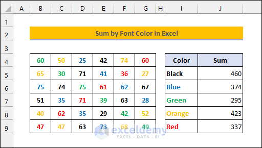
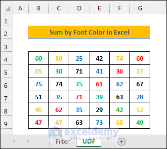
Sum by Font Color in Excel (2 Effective Ways)

This article illustrates how to sum cells by their font color in Excel. Here’s a dataset with various values colored in random colors. We’ll sum the values based on the font color.

Download the Practice Workbook

Sum by Font Color.xlsm

2 Effective Ways to Sum by Font Color in Excel

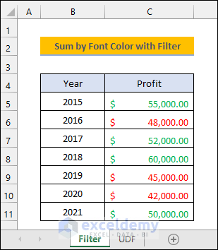
Method 1 – Sum by Font Color with SUBTOTAL and Filter

Consider the following dataset with profit values either being green or red (which could mean positive or negative). We’ll sum values that share a color.

Steps

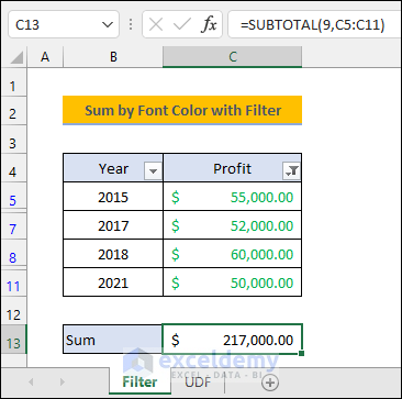
Enter the following formula in cell C13. The 9 in the formula refers to the SUM function.

=SUBTOTAL(9,C5:C11)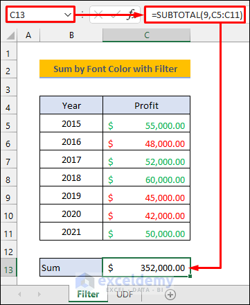

Select anywhere in the dataset.
Press Ctrl + Shift + L to apply a Filter on the dataset.
You will see the filter buttons at the lower right corners of the header cells as shown in the picture below.

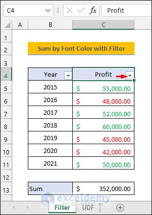
Filter the dataset by a particular color using the filter button as shown below.

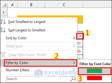
You will get the partial sum based on the color.

Similar Readings

Method 2 – Sum by Font Color with a User Defined Function (UDF) in Excel

We’ll use a function to sum the various values since they are in both rows and columns.

Steps

Save the workbook as a macro-enabled workbook.
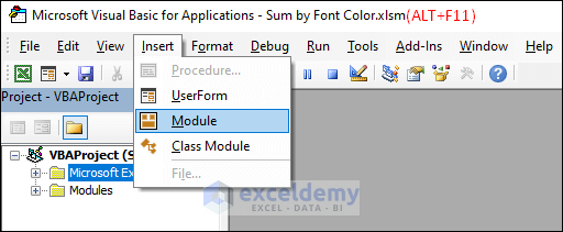
Press Alt + F11 to open the VBA window.
Select Insert and Module as shown in the picture below. This will create a new blank module.

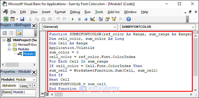
Copy the code given below.

Function SUMBYFONTCOLOR(ref_color As Range, sum_range As Range)
Dim cell_color, sum_color As Long
Dim Cell As Range
Application.Volatile
sum_color = 0
cell_color = ref_color.Font.ColorIndex
For Each Cell In sum_range
If cell_color = Cell.Font.ColorIndex Then
sum_cell = WorksheetFunction.Sum(Cell, sum_cell)
End If
Next Cell
SUMBYFONTCOLOR = sum_cell
End Function

Paste the copied code into the module window.

Go back to your worksheet.
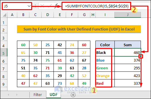
Write the desired color names in cells I5:I9. Change their font colors according to the color.
Enter the following formula in cell J5 and use the Fill Handle icon to apply the formula to the cells below.

=SUMBYFONTCOLOR(I5,$B$4:$G$9)

Finally, you will get the following result.

If you change the font color of any cells within the range, the result won’t update.
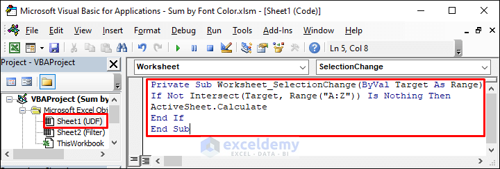
Copy the following code that enables auto-updates.

Private Sub Worksheet_SelectionChange(ByVal Target As Range)
If Not Intersect(Target, Range("A:Z")) Is Nothing Then
ActiveSheet.Calculate
End If
End Sub

Go back to the VBA window.
Double-click on the worksheet named UDF. This will open a blank window.
Paste the copied code into that window.

You can change the font colors and click away to update the results.

Explanation of the VBA Code

Function SUMBYFONTCOLOR(ref_color As Range, sum_range As Range)
This public function will take two arguments. The ref_color argument will take the font color from the reference cell. We will sum the cell values based on their font colors within the range referred to by the sum_range argument.

Dim cell_color, sum_color As Long
Dim Cell As Range
Declaring necessary variables.

Application.Volatile
This code line forces excel to recalculate whenever the user makes any changes.

sum_color = 0
Defining the initial value for the variable.

cell_color = ref_color.Font.ColorIndex
The cell_color variable stores the font color of the cell referred by the ref_color argument.

For Each Cell In sum_range
This For Loop will execute the next code lines through each cell within the range referred by the sum_range argument.

If cell_color = Cell.Font.ColorIndex Then
Only if the font color of a cell within the sum_range matches with the font color of the cell referred by the ref_color argument then the next code lines will execute.

sum_cell = WorksheetFunction.Sum(Cell, sum_cell)
This code line activates the SUM function to add the cell values with matching font colors.

SUMBYFONTCOLOR = sum_cell
This code line stores the sum so that the function can return this value.

Private Sub Worksheet_SelectionChange(ByVal Target As Range)
This private subject procedure works only if any changes occurs within the particular worksheet.

If Not Intersect(Target, Range(“A:Z”)) Is Nothing Then
This code line ensures that the next code line will execute only if the user makes any changes within the defined range (A:Z).

ActiveSheet.Calculate
This forces a recalculation of all formulas within active the worksheet so that changes are updated.

Get FREE Advanced Excel Exercises with Solutions!

2 Comments

Paul Mar 8, 2023 at 7:59 AM

Hello, is there a way to apply a date condition? Let’s say I want to count font colour but only between two dates, from the example above let’s say from B3 to G3 there’s dates 3/1/23, 3/2/23, 3/3/23 etc, I only want to count font color between first of the month and today’s date. Is there a way to do it?
- Reply
  Aniruddah Alam Mar 9, 2023 at 3:46 PM
  Thank you Paul for reaching out. For your special case, it is possible to make a custom function that sums up all the numbers within a specific date range and has specific font color. To do this, we have to pass two more arguments in the function (Starting_Date & Ending_Date). For illustration, I have taken another data set that contains Dates on the column header as you suggested.
  
  I have written another code to create a User-defined Function named SumByDateColor.
```
Function SumByDateColor(starting_date As Variant, ending_date As Variant, ref_color As Range, sum_range As Range) As Double
    Dim cell_color As Long, sum_cell As Double
    Dim cell As Range
    Application.Volatile
    sum_cell = 0
    cell_color = ref_color.Font.colorIndex
    'iterating through columns
    For i = 1 To sum_range.Columns.Count
        If (sum_range.Cells(1, i) >= starting_date And sum_range.Cells(1, i) <= ending_date) Then
            For j = 2 To sum_range.Rows.Count
            'iterating through rows from each column
                Set cell = sum_range.Cells(j, i)
                    If cell_color = cell.Font.colorIndex Then
                        sum_cell = sum_cell + cell.Value
                    End If
            Next j
        End If
    Next i
    SumByDateColor = sum_cell
End Function
```
  In cell L5, if we apply the function, it will return the sum of all the black font numbers from the first three columns (From 03/03/23 to 03/05/23).
  =SUMBYDateColor(I5,J5,K5,$B$4:$G$10)
  
  In this way, we can apply the function for L6: L9 as well and get the following result.
  
  I hope it will solve your problem. If you have any further queries or need the work file, you can ask in our Exceldemy Forum.
  Regards
  Aniruddah

Sum by Font Color in Excel (2 Effective Ways)

Download the Practice Workbook

2 Effective Ways to Sum by Font Color in Excel

Method 1 – Sum by Font Color with SUBTOTAL and Filter

Method 2 – Sum by Font Color with a User Defined Function (UDF) in Excel

Related Articles

Leave a reply Cancel reply