For the sample data, we have a Sales Report of a certain fruit business.
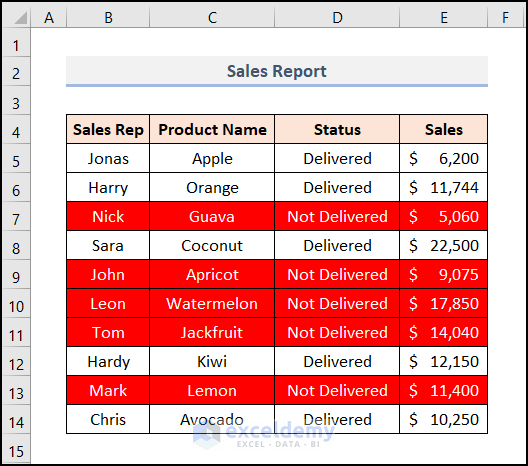
Rows containing undelivered products (marked “Not Delivered“) are colored red. We’ll calculate the total sales amount for these red-colored cells.
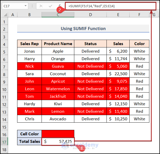
Method 1 – Using SUMIF Function to Sum If Cell Color Is Red in Excel
Steps
- Add a new column (Column F) and label it “Color” in cell F4.
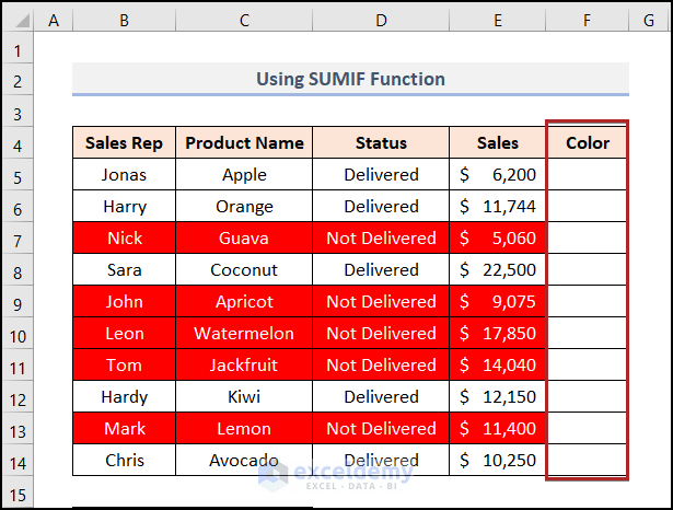
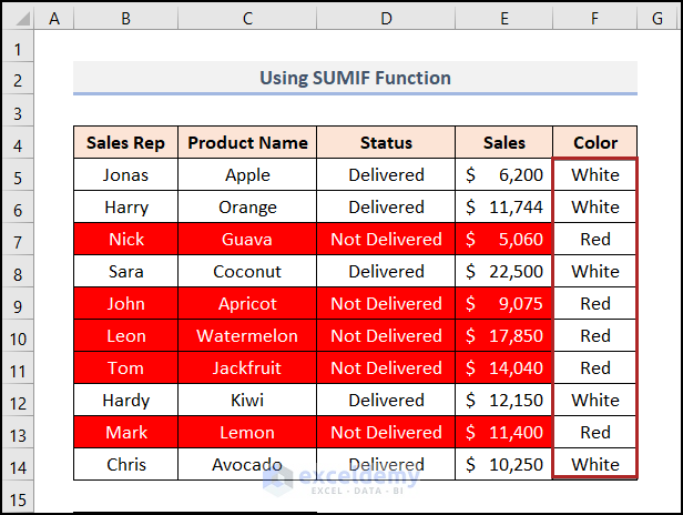
- In Column F, manually enter the background color of each row (e.g., “White” for non-red and “Red” for red).
- Select cells in the B16:C17 range and create an output section in the selected area as shown in the image below.
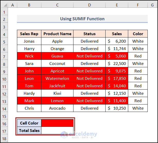
- Select cell C17 and enter the following formula:
=SUMIF(F5:F14,"Red",E5:E14)
- Press Enter to display the sum of sales for red-colored cells.
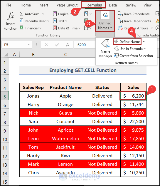
Method 2 – Using GET.CELL Function to Sum If Cell Color Is Red in Excel
- Select cell E5.
- Go to the Formulas tab and click on Defined Names.
- Select Define Name from the drop-down menu.
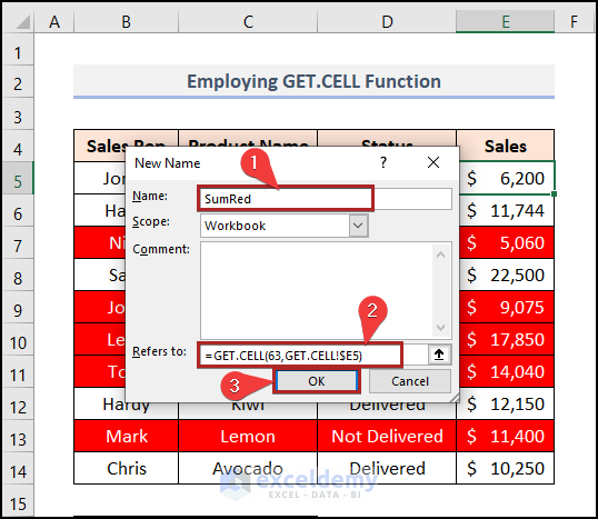
- In the New Name dialog box, enter SumRed in the Name box.
- In the Refers to box, enter the following formula:
=GET.CELL(63,GET.CELL!$E5)
- Click OK.
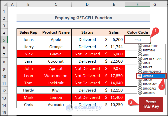
- Create a new column (Column F) and label it Color Code in cell F4.
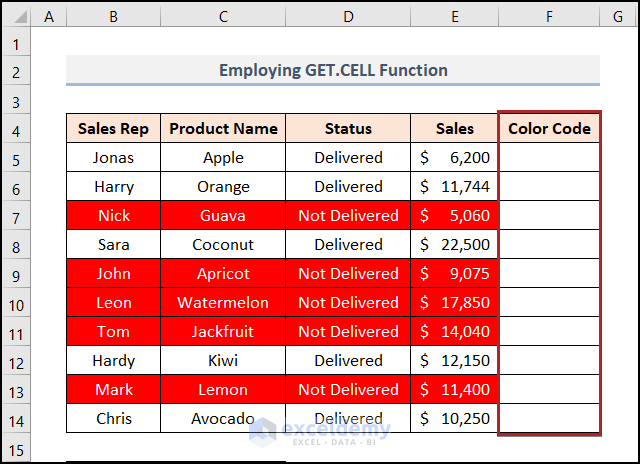
- Select cell F5 and start typing the function name (SumRed). Excel will show a list of suggested functions.
- Select the function SumRed and press the TAB key on the keyboard.
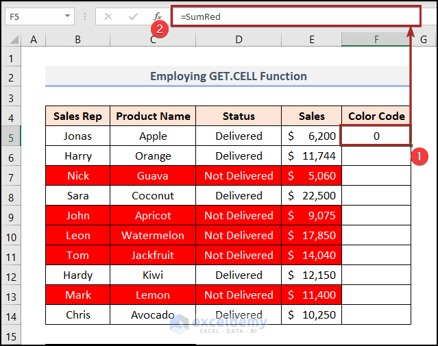
- Hit the ENTER key.
- Cell F5 will have 0 as output (O is the color code of No Fill background color).
- Drag the Fill Handle icon down Column F to copy the formula to all cells.
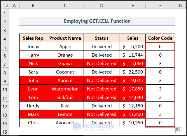
Note: Cells with no background color will have a color code of 0, while cells with red background color will have a color code of 3.
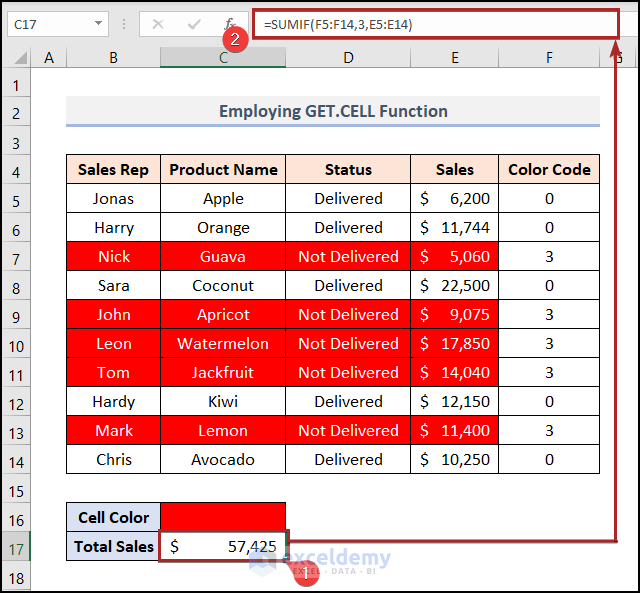
- Select cell C17 and enter the following formula.
=SUMIF(F5:F14,3,E5:E14)
- Press the ENTER key to display the sum of sales for red-colored cells.
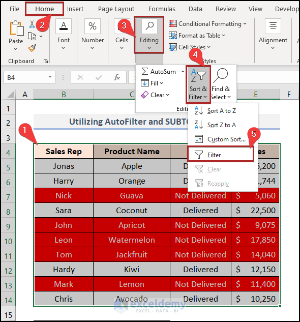
Method 3 – Utilizing AutoFilter and SUBTOTAL Function to Sum if Cell Color is Red in Excel
Steps
- Select cells in the B4:E14 range.
- Go to the Home tab.
- Click on the Editing group.
- Select the Sort & Filter drop-down menu.
- Choose Filter from the drop-down list.
- Filter arrows appear next to headers.
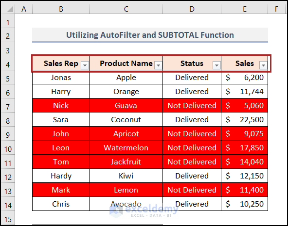
- Click on the filter arrow next to the Sales heading.
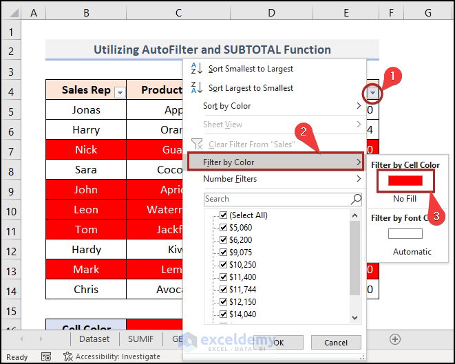
- A context menu will appear beside the icon.
- Select the Filter by Color option.
- Select the red color rectangle.
- Only red-colored rows will now be visible. Other rows are hidden.
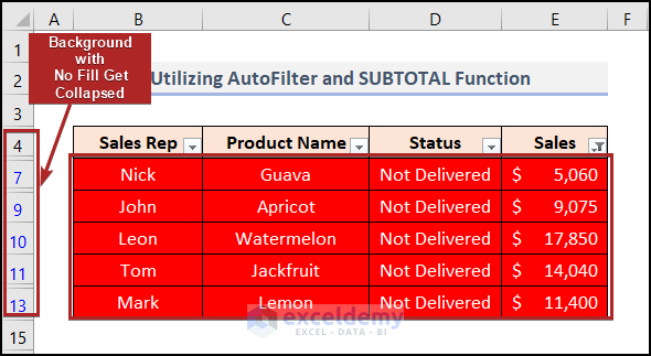
- Select cell C17 and enter the formula:
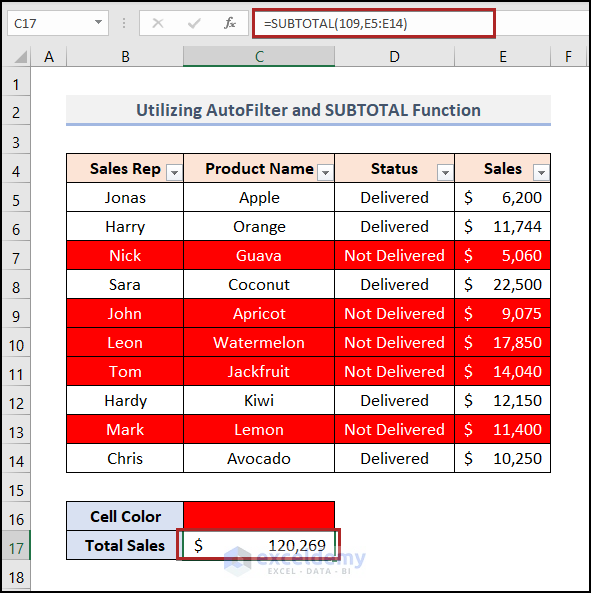
=SUBTOTAL(109,E5:E14)
- Hit the ENTER key.
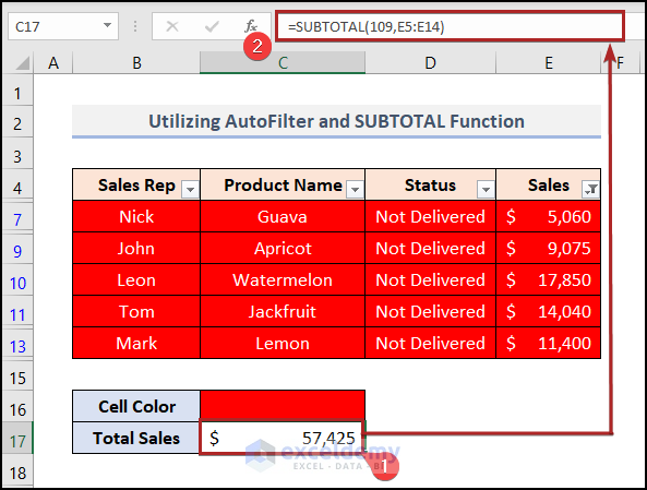
It will give the sum of the visible cells. The hidden cells aren’t included in the calculation.
- Click the filter arrow next to Sales again.
- From the drop-down menu select Clear Filter From “Sales”.
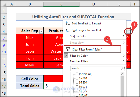
- Hidden rows will now be visible.
- The formula remains unchanged, but the Total Sales sum will adjust to include all rows (including previously hidden ones).
Method 4 – Applying VBA Code to Sum if Cell Color is Red in Excel
Steps
- Press the ALT + F11 key.
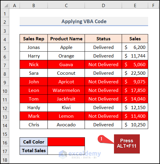
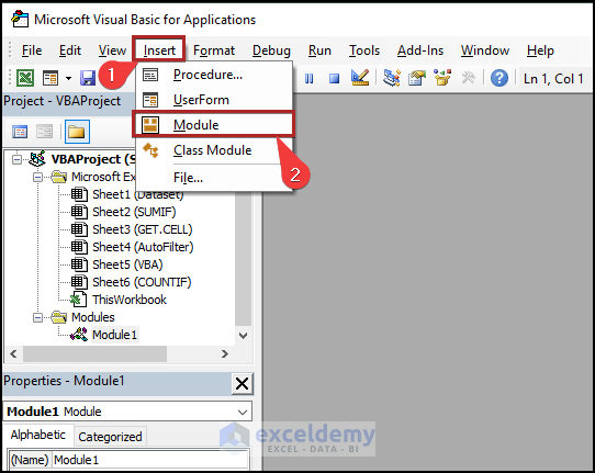
- Microsoft Visual Basic for Applications window will open.
- Go to Insert tab.
- Select Module.
- In the code module, paste the code below.
Function Sum_Red_Cells(cc As Range, rr As Range)
Dim x As Long
Dim y As Integer
y = cc.Interior.ColorIndex
For Each i In rr
If i.Interior.ColorIndex = y Then
x = WorksheetFunction.Sum(i, x)
End If
Next i
Sum_Red_Cells = x
End Function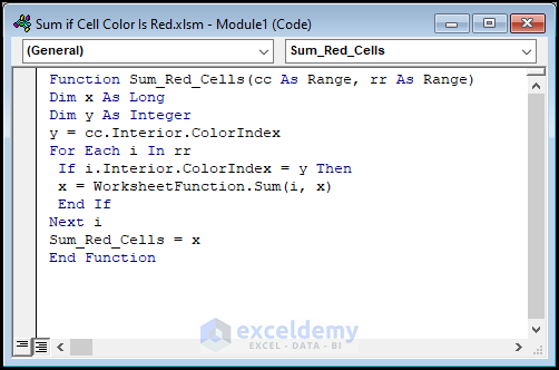
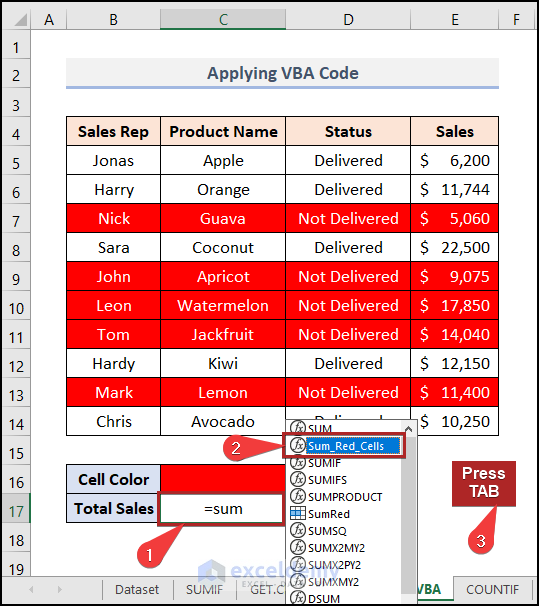
- Return to the worksheet VBA.
- Select cell C17 and start to type the function =sum.
- Select the function Sum_Red_Cells and press the TAB key on the keyboard.
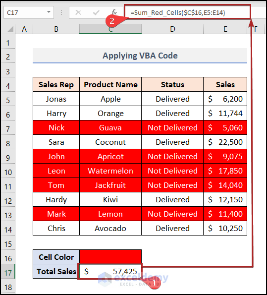
- Enter the required cell reference and cell range(C16, E5:E14) to perform the sum operation.
Download Practice Workbook
Related Articles
- How to Sum Colored Cells in Excel Without VBA
- How to Sum Random Cells in Excel
- How to Ignore Blank Cells in Excel Sum
- [Solved!] Currency Sum Not Working in Excel
<< Go Back to Sum in Excel | Calculate in Excel | Learn Excel
Get FREE Advanced Excel Exercises with Solutions!
