How to Detect If a Sum Is Not Working in Excel
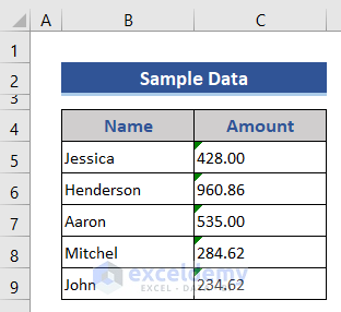
We have the following dataset to get the sum.
- We applied the SUM function on Cell C10.
=SUM(C5:C9)
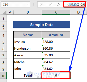
- The result is zero, instead of the expected value.
- Let’s check the data of Range C5:C9.
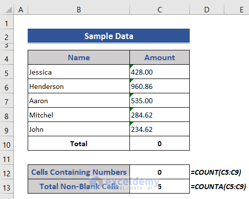
The COUNTA function checks the numbers of non-empty cells, and the COUNT function checks cells containing numbers only. Both of the functions count based on the given criteria.
We can see no cells contains numbers. They may be in text or other custom formats.
- To check the format of the data, go to the Number Format section of the Number group.
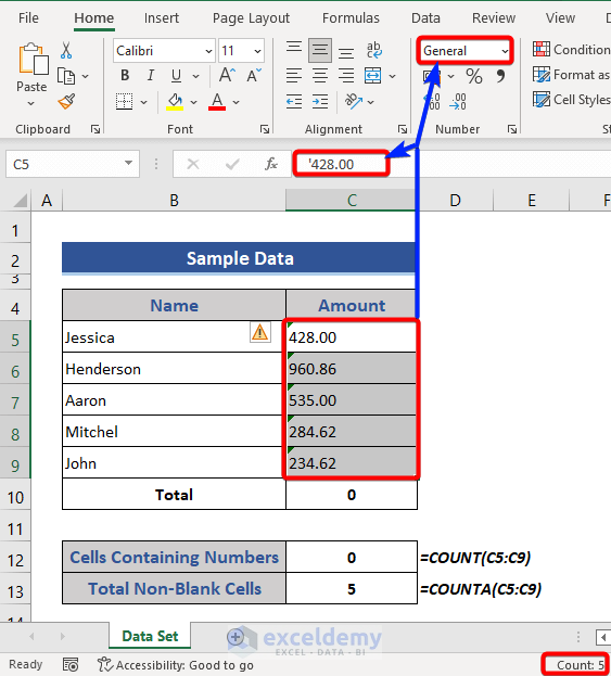
We can see the given data are in General format. There is a leading apostrophe symbol at the start of the number. Because of this, an error is showing in each cell of the dataset. The status bar is also not showing the total, only counting the cells.
Currency Sum Is Not Working in Excel: 6 Solutions
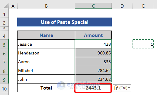
Solution 1 – Use Paste Special Multiplication to Convert Numbers into Number Format
Steps:
- Go to any blank cell of the dataset and insert 1.
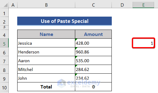
We will use this 1 to multiply the given data. As we are using 1, the values will not change.
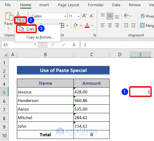
- Select the cell that contains 1.
- Select the Copy option from the Clipboard group. You can also use Ctrl + C to copy data.
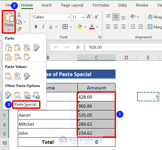
- Select Range C5:C9.
- Go to Paste from the Clipboard group.
- Select the Paste Special option. Ctrl + Alt+ V is the keyboard shortcut for Paste Special.
- The Paste Special window appears.
- Mark Values from the Paste segment and Multiply from the Operation segment.
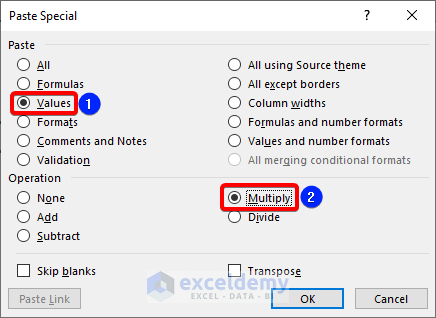
- Press the OK button and look at the dataset.
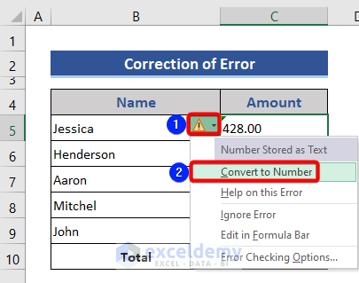
Solution 2 – Use Error Checking
Steps:
- Click on Cell C5.
- You will see an error notification on the left side.
- Click on the down arrow.
- Choose the Convert to Number option.
- Look at the dataset.
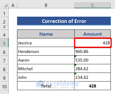
The error has been removed.
- Remove the errors of the rest of the data.
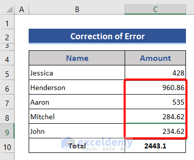
After removing all the errors, we get the sum successfully.
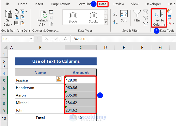
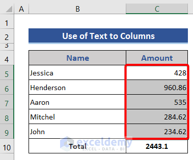
Solution 3 – Use the Text to Columns Wizard to Convert Numbers in Text to Number Format
Steps:
- Select Range C5:C9.
- Select Text to Columns from the Data tab.
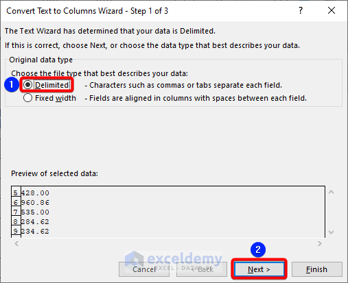
- The 1st step of the Convert Text to Columns Wizard window appears.
- Mark the Delimited option, then click on the Next button.
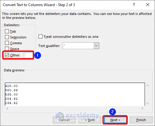
- The 2nd step appears.
- Mark Other and put the apostrophe(‘) symbol on the box.
- Click on the Next button.
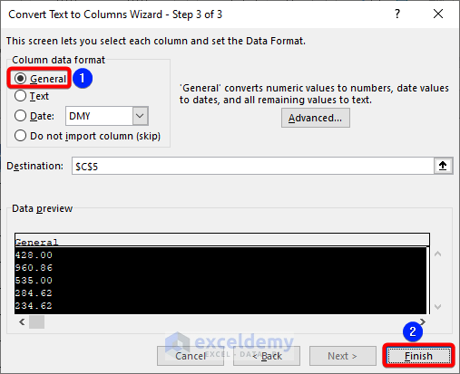
- Choose the General option.
- Click on the Finish option.
- Look at the dataset.
Solution 4 – Use Flash Fill to Get the Currency Sum
Steps:
- Add a column on the right side.
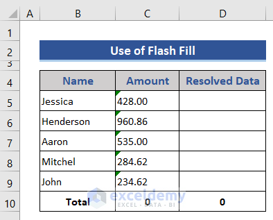
- Type in the data of Cell C5 into Cell D5 manually.
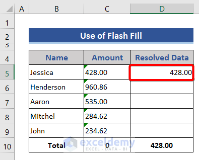
- Select the Range D5:D9.
- Choose Flash Fill of the Data Tools group from the Data tab.
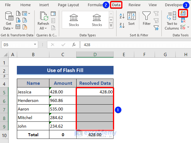
- Look at the dataset.
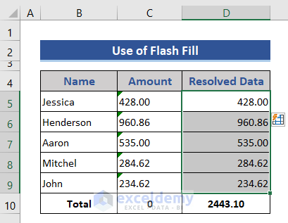
We can see all the errors have been corrected and get the sum. You can use the keyboard shortcut Ctrl + E to apply Flash Fill.
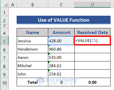
Solution 5 – Use the VALUE Function
The NUMBERVALUE function converts a text to number in a locale-independent manner.
Steps:
- Go to Cell D5 and put in the following formula.
=VALUE(C5)
- Press the Enter button and drag the Fill Handle icon.
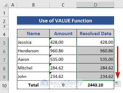
We get the currency sum accurately. We can also use the NUMBERVALUE function instead of the VALUE function. The formula will look like this:
=NUMBERVALUE(C5)
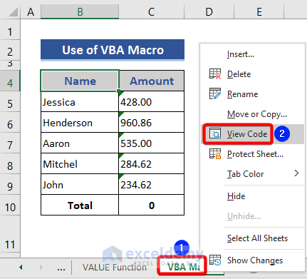
Solution 6 – Use Excel VBA Code to Get the Currency Sum
Steps:
- Go to the bottom of the worksheet containing the sheet name section.
- Right-click on the sheet name.
- Select the View Code option from the Context Menu.
- The VBA window appears.
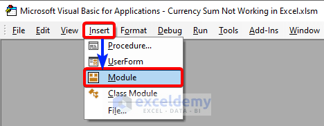
- Choose the Module option from the Insert tab.
- Put the following VBA code on the module.
Sub Solve_Errors()
Dim range_1 As Range
On Error Resume Next
Set range_1 = Selection.SpecialCells(xlCellTypeConstants, 23)
On Error GoTo errHandler
If Not range_1 Is Nothing Then
Cells.SpecialCells(xlCellTypeLastCell).Offset(0, 1).Copy
range_1.PasteSpecial Paste:=xlPasteValues, Operation:=xlPasteSpecialOperationAdd
Else
MsgBox "No Constant Found"
End If
exitHandler:
Application.CutCopyMode = False
Set range_1 = Nothing
Exit Sub
errHandler:
MsgBox "Change Not Possible"
Resume exitHandler
End Sub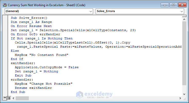
- Select the Range C5:C9.
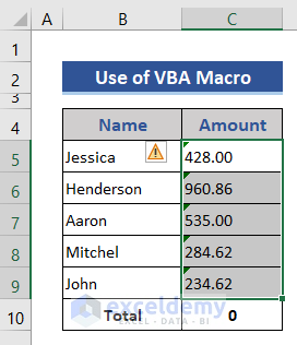
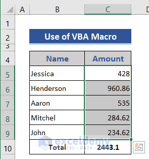
- Run the VBA code by pressing the F5 button.
Download the Practice Workbook
Related Articles
- How to Sum Random Cells in Excel
- How to Sum in Excel If the Cell Color Is Red
- How to Sum Colored Cells in Excel Without VBA
- How to Ignore Blank Cells in Excel Sum
<< Go Back to Sum in Excel | Calculate in Excel | Learn Excel
Get FREE Advanced Excel Exercises with Solutions!
