If you are looking for Excel sum visible cells with criteria, you have come to the right place. Here, we will walk you through 5 easy and effective methods to do the task smoothly.
How to Sum Visible Cells with Criteria in Excel: 5 Methods
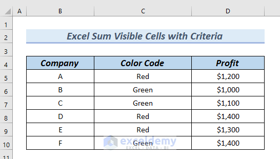
The following dataset has the Company, Color Code, and Profit Columns. Using this dataset, we will go through 5 methods for Excel sum visible cells with criteria.
Here, we used Microsoft Excel 365. You can use any available Excel version.
1. Use of SUBTOTAL Function to Sum Visible Cells with Criteria
In this method, we will use the SUBTOTAL function to sum visible cells with criteria. Here, first, we will create a table using the following dataset, and after that, we will show the sum of the Profit based on the Green color code only.
Let’s go through the following steps to do the task.
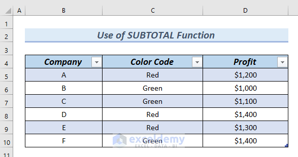
Step-1: Inserting Table
In this step, we will insert a Table.
- First of all, we will select the entire dataset from cells B4:D10.
- After that, we will go to the Insert tab >> select Table.

After that, a Create Table dialog box will appear.
Make sure My table has headers marked.
- Then, click OK.

As a result, you can see the Table.
Step-2: Using SUBTOTAL Function
In this step, we will use the SUBTOTAL function to sum visible cells with criteria.
- In the beginning, we will type the following formula in cell D11.
=SUBTOTAL(9,[Profit])Here, the SUBTOTAL function yields the summation of the Profit column.
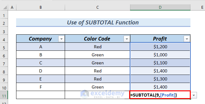
- After that, press ENTER.
As a result, you can see the result in cell D11.
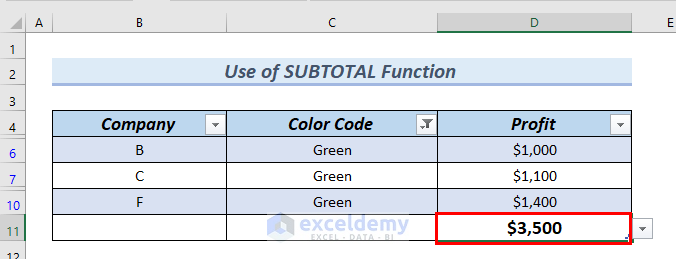
Next, we will Filter the Table and we will keep only the Green color code.
- Afterward, we will click on the drop-down arrow of the heading Color Code in cell C4.

- Next, we will unmark Red color >> click OK.

Therefore, you can see the Table now shows a Green color code only.
Along with that, cell D11 shows the sum of the visible cells only.
2. Applying SUMIF and AGGREGATE Functions
In this method, we will use the SUMIF and AGGREGATE functions to sum visible cells with criteria.
Here, we will find the Profit based on the color Red.

Steps:
- In the beginning, we will insert Assistant Column into the dataset.
- After that, we will type the following formula in cell E5.
=AGGREGATE(9,5,D5)The AGGREGATE function yields an aggregate in a data table.
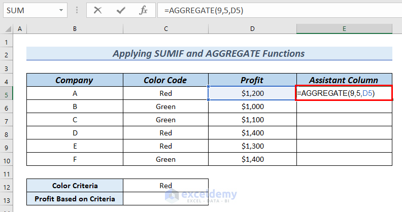
- Afterward, press ENTER.
Then, you can see the result in cell E5.
- Furthermore, we will drag down the formula with the Fill Handle tool.

As a result, you can see the complete Assistant Column.
- Moreover, we will type the following formula in cell C13.
=SUMIF(C5:C10,"Red",E5:E10)The SUMIF function yields the summation of the values of a range of cells that meet the criteria we specify.

- At this point, press ENTER.
Therefore, you can see the result in cell C13.

- After that, we followed Step-1 of Method-1 to insert a Table.
Therefore, you can see the Table.
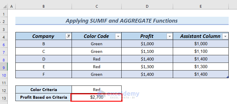
- Next, we will click on the drop-down arrow of the heading Company in cell B4.

- After that, we unmark A >> click OK.

As a result, you can see Company A has been hidden.
Along with that, you can see the sum visible cells with criteria in cell C13.
3. Using Combined Functions
In this method, we will use the combination of SUMPRODUCT, SUBTOTAL, OFFSET, ROW, and MIN functions to sum visible cells with criteria.
- First, we will type the following formula in cell C13.
=SUMPRODUCT(SUBTOTAL(3,OFFSET(C5:C10,ROW(C5:C10)-MIN(ROW(C5:C10)),,1)),(C5:C10=C12)*(D5:D10))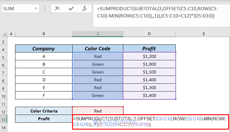
Formula Breakdown
- ROW(C5:C10) → the ROW function yields the row number of a range.
- MIN(ROW(C5:C10)) → the MIN function returns the minimum row number in a sequence.
- Output: 5
- OFFSET(C5:C10,ROW(C5:C10)-MIN(ROW(C5:C10)),,1) → the OFFSET function returns a section from a data set with a specific height and a specific width, situated at a specific number of rows down and a specific number of columns right from a given cell reference.
- SUBTOTAL(3,OFFSET(C5:C10,ROW(C5:C10)-MIN(ROW(C5:C10)),,1)) → the SUBTOTAL function yields the summation of the Profit
- SUMPRODUCT(SUBTOTAL(3,OFFSET(C5:C10,ROW(C5:C10)-MIN(ROW(C5:C10)),,1)),(C5:C10=C12)*(D5:D10)) → the SUMPRODUCT function yields the summation of products of a range.
- Output: $3900
- Explanation: Here, $3900 is the sum of the Profit based on the color RED.
- Afterward, press ENTER.
- As a result, you can see the result in cell C13.

- After that, we followed Step-1 of Method-1 to insert a Table.
Therefore, you can see the Table.
- Next, we will click on the drop-down arrow of the heading Company in cell B4.

- After that, we unmark D >> click OK.

Hence, you can see Company D has been hidden.
In addition, you can see the sum visible cells with criteria in cell C13.

4. Use of SUMPRODUCT, SUBTOTAL, OFFSET, and ROW Functions
In this method, we will use the combination of SUMPRODUCT, SUBTOTAL, OFFSET, and ROW, functions to sum visible cells with criteria.
Here, we will find out the Profit based on the Green color code.

Steps:
- First, we will type the following formula in cell C13.
=SUMPRODUCT(SUBTOTAL(109,OFFSET(D5,ROW(Table137[Profit])-ROW(D5),)),--(Table137[Color Code]=C12))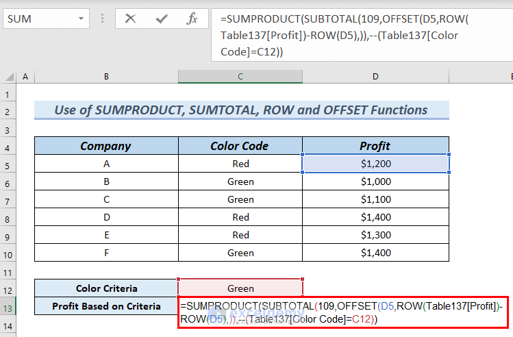
Formula Breakdown
- ROW(Table137[Profit])-ROW(D5) → the ROW function yields the row number of a range.
- OFFSET(D5,ROW(Table137[Profit])-ROW(D5),)) → the OFFSET function returns a section from a data set with a specific height and a specific width, situated at a specific number of rows down and a specific number of columns right from a given cell reference.
- SUBTOTAL(109,OFFSET(D5,ROW(Table137[Profit])-ROW(D5),)) → the SUBTOTAL function yields the summation of the Profit
- SUMPRODUCT(SUBTOTAL(109,OFFSET(D5,ROW(Table137[Profit])-ROW(D5),)),–(Table137[Color Code]=C12)) → the SUMPRODUCT function yields the summation of products of a range.
- Output: $3500
- Explanation: Here, $3500 is the sum of the Profit based on the color Green.
- Then, press ENTER.
Therefore, you can see the result in cell C13.

- At this point, we followed Step-1 of Method-1 to insert a Table.
Hence, you can see the Table.
- Furthermore, we will click on the drop-down arrow of the heading Company in cell B4.

- After that, we unmark B >> click OK.

Hence, you can see Company B has been hidden.
In addition, you can see the sum visible cells with criteria in cell C13.

5. Using Filter Feature and SUBTOTAL Function to Sum Visible Cells with Criteria
In this method, we will use the Filter feature along with the SUBTOTAL function to sum visible cells with criteria.
Steps:
- First, we add the Sales and Total columns into the dataset.
- Then, we select the entire dataset from cells B4:F10.
- After that, from the Data tab >> select Filter.

As a result, you can see the filter icon in the dataset.
- Furthermore, we will click on the drop-down arrow of the heading Color Code in cell C4.

- Then, we will unmark Green >> click OK.

Therefore, you can see the filtered dataset with visible Red color only.
- Next, we will click we will click on the drop-down arrow of the heading Color Code in cell D4

- Next, we unmark $1300 >> click OK.

- Moreover, we type the following formula in cell F5.
=SUBTOTAL(9,D5:E5)Here, the SUBTOTAL function yields the summation of the Profit column.
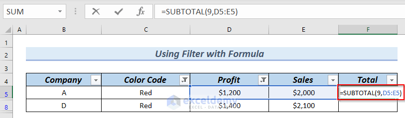
- At this point, press ENTER.
As a result, you can see the result in cell F5.
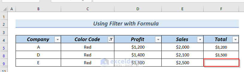
- Furthermore, we will drag down the formula with the Fill Handle tool.

As a result, you can see the sum of the visible cells.
- Next, we will click we will click on the drop-down arrow of the heading Color Code in cell D4.

- Furthermore, we will mark $1300 >> click OK.

Then, you can see that the Total for Profit $1300 is not present in cell F9.
Therefore, you can find the sum visible cells with criteria.
Practice Section
You can download the above Excel file to practice the explained methods.

Download Practice Workbook
You can download the Excel file and practice while you are reading this article.
Conclusion
Here, we tried to show you 5 methods for Excel sum visible cells with criteria. Thank you for reading this article, we hope this was helpful. If you have any queries or suggestions, please let us know in the comment section below.
Related Articles
- How to Sum Random Cells in Excel
- How to Sum in Excel If the Cell Color Is Red
- How to Sum Colored Cells in Excel Without VBA
- [Solved!] Currency Sum Not Working in Excel
- How to Ignore Blank Cells in Excel Sum
<< Go Back to Sum in Excel | Calculate in Excel | Learn Excel
Get FREE Advanced Excel Exercises with Solutions!
