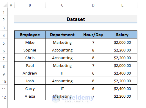
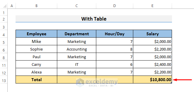
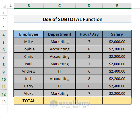
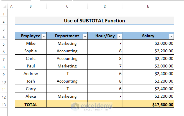
We have a dataset of some employees. It contains four columns: Employee name, Department, working Hours per day, and Salary. Here’s an overview of the dataset we’ll use to sum up values in visible cells only.
Method 1 – Summing Only Visible Cells with a Table in Excel
- Select all data from your datasheet.
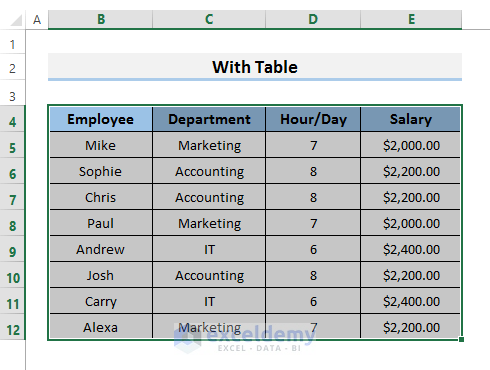
- Go to the Insert tab and select Table.

NOTE: You can also press Ctrl + T.
- Go to the Design ribbon and select Total Row.
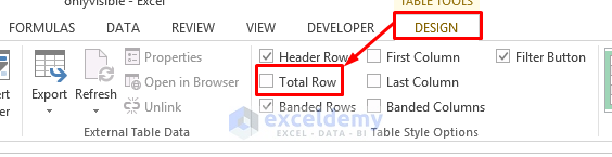
- This will insert a row of the totals. We will see the sum there.
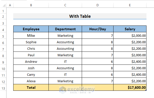
- If we hide some rows, the value of the Total Row will automatically change and provide the sum of the visible cells only. We hid the 7th, 9th, and 10th row, and the sum for the visible cells appeared in the last row.
Read More: Sum to End of a Column in Excel
Method 2 – Using the AutoFilter to Sum Only Visible Cells in Excel
Case 2.1 – Use the SUBTOTAL Function
- Select the entire range of cells in the dataset.
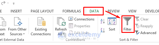
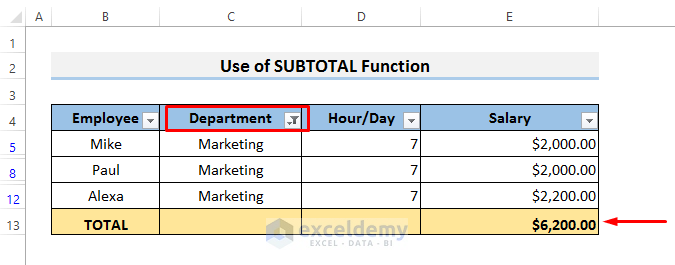
- Go to the Data ribbon and select Filter.
- Select cell E13 and copy the following formula.
=SUBTOTAL(109,E5:E12)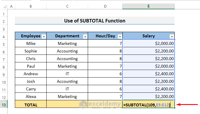
- Press Enter to see the result.
- If we filter any column, the result of the sum will change accordingly and display the sum of visible cells.
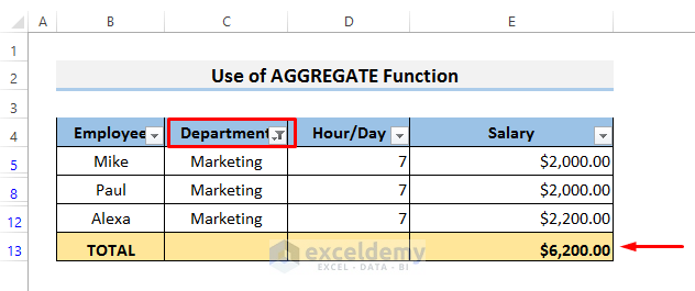
Case 2.2 – Use the AGGREGATE Function
- Apply Filter to the entire dataset.
- Select Cell E13.
- Copy the following formula into the cell:
=AGGREGATE(9,5,E5:E12)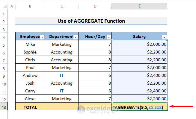
- Press Enter.
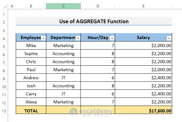
- If we filter any columns, it will only show the sum of the visible cells.
Case 2.3 – Use AutoSum
- Apply a Filter to the dataset.
- Select Cell E13.
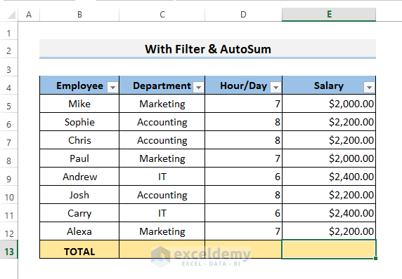
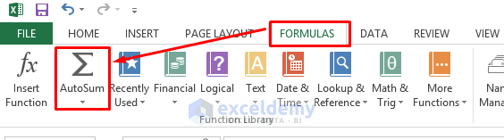
- Go to the Formulas ribbon and select AutoSum.
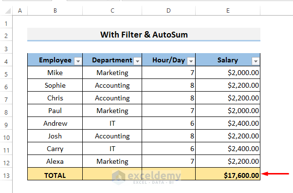
- This will sum the Salary Column and show it in the cell.
Read More: How to Sum Filtered Cells in Excel
Method 3 – Finding a Sum for Visible Cells with a User-Defined Function
- Go to the Developer ribbon and select Visual Basic.

- The Microsoft Visual Basic window will appear. Insert a Module and copy the following code into it:
Function ONLYVISIBLE(CellRng As Range) As Double
Dim x As Range
Dim SumUp As Double
For Each x In CellRng
    If x.Rows.Hidden = False And x.Columns.Hidden = False Then
        SumUp = SumUp + x.Value
    End If
Next
ONLYVISIBLE = SumUp
End Function- Select Cell E13 and copy the following formula.
=ONLYVISIBLE(E5:E12)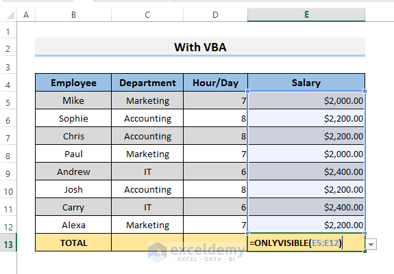
- Press Enter.
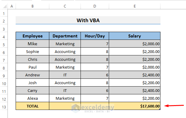
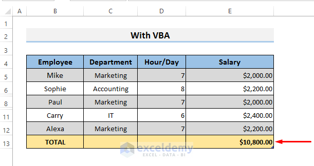
- If we hide some rows, the sum will adjust accordingly.
Read More: How to Sum Random Cells in Excel
Method 4 – Applying the Excel SUMIF Function to Add Visible Cells
- Add two new columns to the previous dataset: a Yes/No Column D and a Helper Column F.
- Select Cell F5 and copy the following formula into it.
=AGGREGATE(9,5,E5)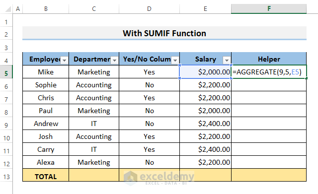
- Press Enter. This just sums up Cell E5 and displays the result. Use the Fill Handle to fill the column.
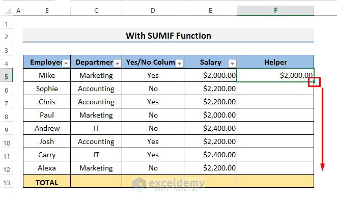
- We will get all the values in the Helper Column.
- Input the following formula in cell E13:
=SUMIF(D5:D12,”Yes”,F5:F12)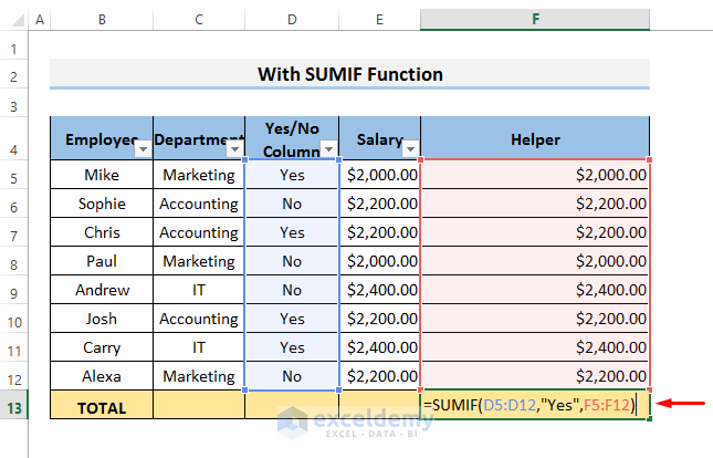
- This will search for Yes in the range D5 to D12 and sum the respective salary if the check yields TRUE.
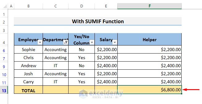
- If we use a Filter, it will only display the sum of the rows if its respective status is Yes.
Read More: Excel Sum If a Cell Contains Criteria
Download Practice Workbook
Download this workbook and practice.
Further Readings
- How to Sum Columns in Excel
- Sum Multiple Rows and Columns in Excel
- How to Sum Colored Cells in Excel
- Calculate Cumulative Sum in Excel
- How to Add Multiple Cells in Excel

