The following picture shows the cumulative sum obtained by using one of the methods.
9 Ways to Perform Cumulative Sum in Excel
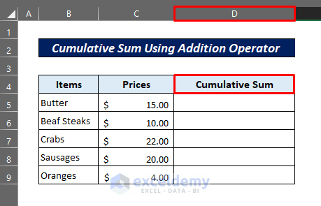
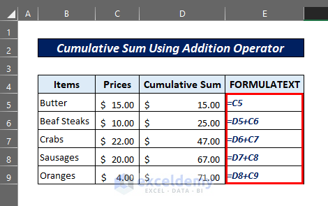
Method 1 – Cumulative Sum Using the Addition Operator
We have a price list of grocery items and want to calculate the cumulative sum in column D.
Steps
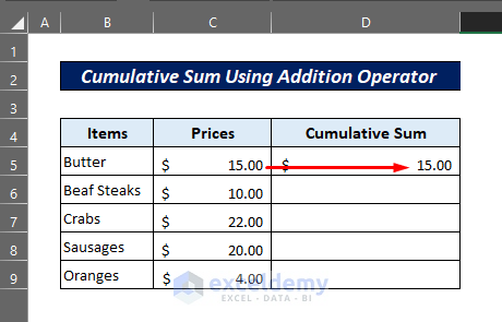
- Enter the following formula in cell D5:
=C5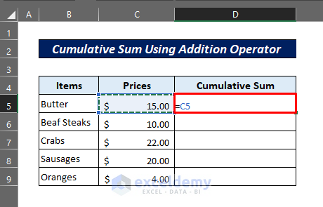
- It gives the same value in Cell D5 as in C5.
- Enter the formula given below in cell D6:
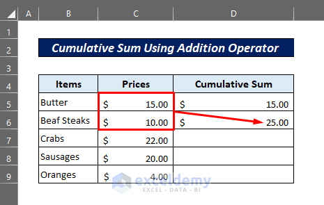
=D5+C6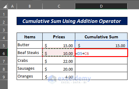
- This will give the cumulative sum of the first two values.
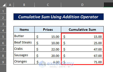
- Continue this formula to the entire column using the Fill Handle tool.
- You will get the cumulative sum as follows.
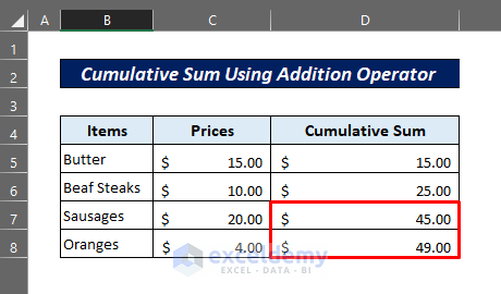
Note: If any of the data rows gets deleted, you will get an error for the next rows.

- If a row is deleted, copy the formula again to those cells.
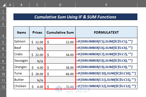
- Here is the final result with the FORMULATEXT function showing what happens in those D cells.
Read More: Sum Formula Shortcuts in Excel
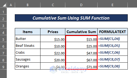
Method 2 – Cumulative Sum Using the Excel SUM Function
Steps
- Enter the following formula in cell D5:
=SUM(C5,D4)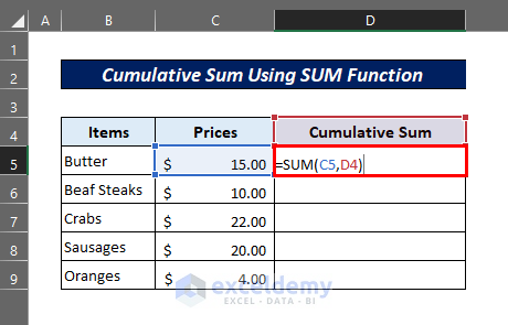
- Apply this formula to the next cells by pulling the Fill-handle icon all the way.

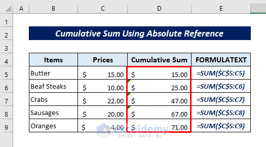
Method 3 – Cumulative Sum Using an Absolute Reference with the SUM Function
Steps
- Enter the following formula in the cell D5:
=SUM($C$5:C5)It makes cell C5 an absolute reference as the starting point.
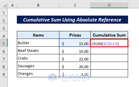
- Copying this formula to the other cells gives the desired result as shown below.
Read More: [Fixed!] Excel SUM Formula Is Not Working and Returns 0
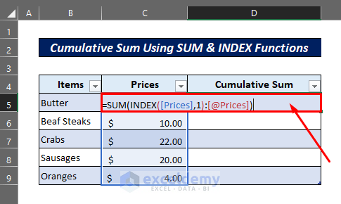
Method 4 – Calculate the Running Total by Using SUM and INDEX Functions
Steps
- Convert the range into a table by pressing Ctrl + T.
- Enter the following formula in cell D5:
=SUM(INDEX([Prices],1):[@prices])The first cell of the second column of the table is created as a reference by the INDEX function as 1 is the row_num argument.
- Applying this formula to the entire column yields the following result.
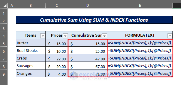
4. Although this method is a little complex to understand, it works great for tabular data.
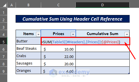
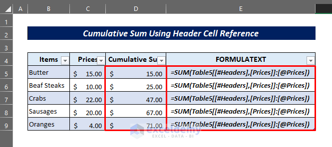
Method 5 – Perform Chain Summation Using an Excel Table
Steps
- Convert the dataset into a table.
- Enter the following formula in cell D5:
=SUM(Table5[[#Headers],[Prices]]:[@Prices])You can type the blue-colored part of the formula by clicking on cell C4.
- Copy this formula to the next cells and get the result as follows.
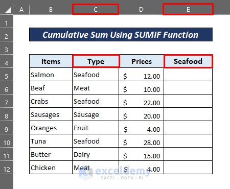
Method 6 – Conditional Cumulative Sum Using the SUMIF Function
We want to get the cumulative sum only for the seafood items.
Steps
- Enter the following formula in cell E5:
=SUMIF($C$5:C5,$E$4,$D$5:D5)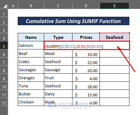
- Copy the formula down to the entire column.
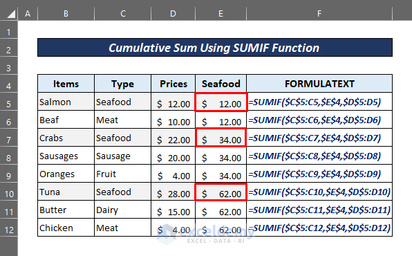
Read More: Sum Cells in Excel: Continuous, Random, With Criteria, etc.
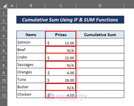
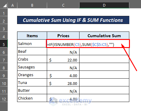
Method 7 – Cumulative Sum Using IF and SUM Functions Ignoring Text Values
Consider the following data where some values are in the text format.
Steps
- Enter the following formula in cell D5:
=IF(ISNUMBER(C5),SUM($C$5:C5),"")The SUM function in this formula only accepts values from the cells of column C if the ISNUMBER function verifies it as a number.
- Apply this formula down to all the other cells.
Read More: How to Sum Cells with Text and Numbers in Excel
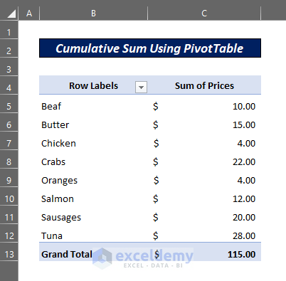
Method 8 – Cumulative Sum Using a Pivot Table
Suppose you have a PivotTable as follows.
Steps
- Click here to learn how to insert a PivotTable.
- Click anywhere in the PivotTable area.
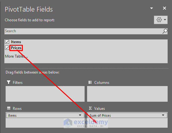
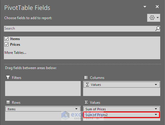
- In the PivotTable Fields, drag the Prices field in the Value area as shown in the following picture.
- It will create another column named ‘Sum of Prices2’.
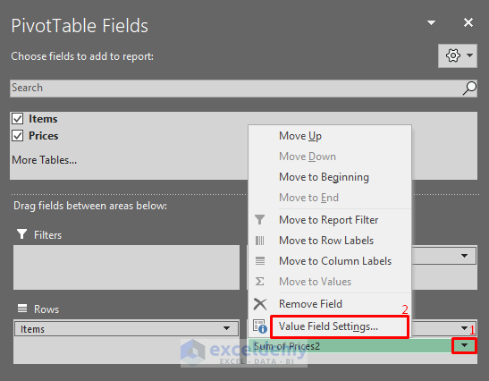
- Click on the dropdown arrow and go to the Value Field Settings.
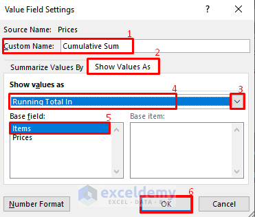
- Change the custom name to Cumulative Sum or as you wish.
- Click on the Show values as field.
- Select Running Total In from the dropdown list.
- Keep the Base field as Items and hit OK.
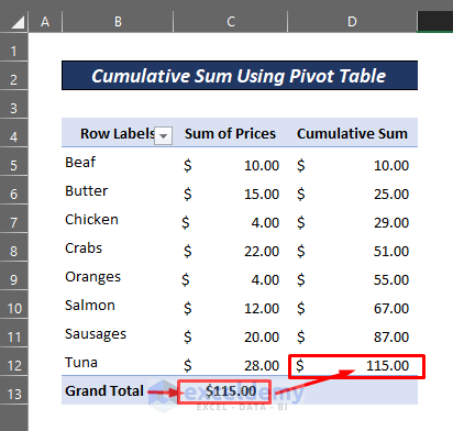
- You will get the cumulative sum in a new column in your Pivot Table.
Read More: Shortcut for Sum in Excel
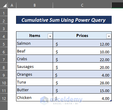
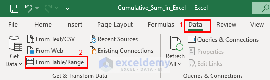
Method 9 – Cumulative Sum Using the Power Query Tool
Consider the following Excel table.
Steps
- Go to the Data tab and click on From Table/Range.
- It will open a table in the Power Query Editor.
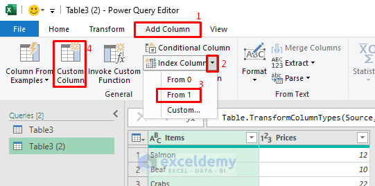
- From the Add Column tab, click on the small arrow right next to Index Column and choose From 1.
- Click on the Custom Column icon.
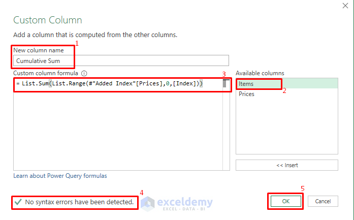
- Change the New Column Name in the Custom Column dialog box to Cumulative Sum.
- Keep the ‘Items’ field selected in the Available columns field.
- Use the following formula in the Custom column formula field.
=List.Sum(List.Range(#"Added Index"[Prices],0,[Index]))- Hit the OK button. This will generate a new column named Cumulative Sum.
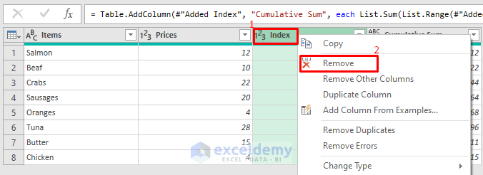
- Right-click on the Index column and remove it.
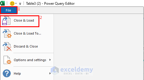
- From the File menu, choose Close & Load.
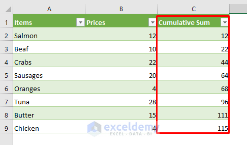
- You will get the cumulative sum as follows.
Read More: Excel Sum If a Cell Contains Criteria
Download the Practice Workbook
Related Articles
- How to Use VLOOKUP with SUM Function in Excel
- Sum All Matches with VLOOKUP in Excel
- Vlookup and Sum Across Multiple Sheets in Excel
- How to Sum If Cell Contains Specific Text in Excel
- How to Sum Top n Values in Excel
- How to Add Percentages to Numbers in Excel

