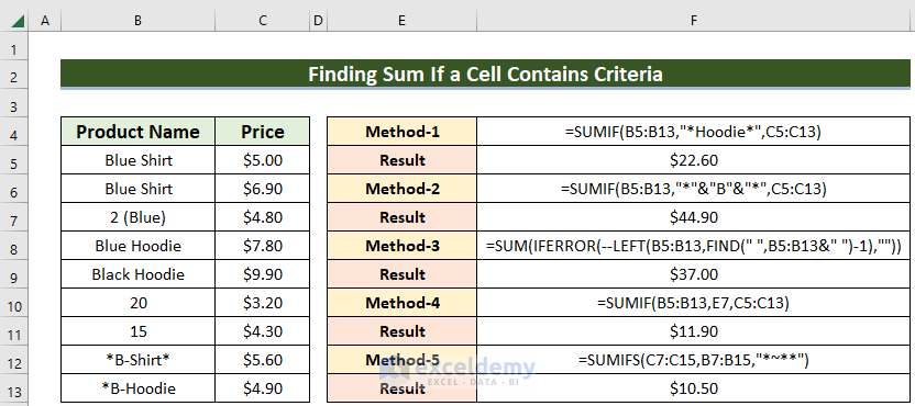
Here’s an overview of all the methods you can use to sum cells based on different criteria options.
Download the Practice Workbook
You can download the workbook from here to follow along.
Introduction to SUMIF and SUMIFS Functions in Excel
The SUMIF Function
Objective:
Adds the cells specified by a single given condition or criteria.
Formula Syntax:
=SUMIF(range, criteria, [sum_range])Arguments:
range= the range of the data.
criteria= the condition based on which summation will take place.
sum_range= the range of data whose specific cells based on criteria will be summed up.
The SUMIFS Function
Objective:
Adds the cells if respective cells from specific ranges each fulfill a condition or criteria.
Formula Syntax:
=SUMIFS(sum_range, criteria_range1, criteria1, [criteria_range2], [criteria2],…)Arguments:
sum_range= the range of data whose specific cells based on criteria will be summed up.
set of criteria_range (criteria_range1, criteria_range2…)= the range of the data where the condition will be applied.
set of criteria (criteria1, criteria2…)= the condition to apply.
Read More: SUMIF vs SUMIFS in Excel (A Comparative Analysis)
5 Examples for Finding a Sum If a Cell Contains Criteria
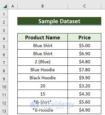
We will use the following dataset in the following examples. The dataset contains 2 columns with the Product Name and Price of products of a company. The Product Name column contains varieties of names with texts, numbers, and asterisks.
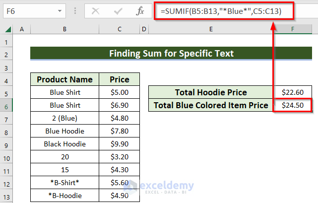
Method 1 – Finding a Sum If a Cell Contains Specific Text
Let’s get the sum of the price of products having the specific text “Hoodie” within the name.
Steps:
- Copy the following formula in Cell F5:
=SUMIF(B5:B13,"*Hoodie*",C5:C13)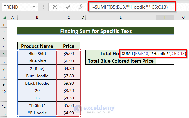
- Press Enter.
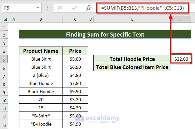
There are 3 names of products with this specific text in the dataset. The result shows the sum of the price of those 3 products.
We can also see results for the name of products having specific text “Blue”. Use "*Blue*" in the given formula instead of "*Hoodie*" and press Enter.
How Does the Formula Work:
Here, the first argument of the SUMIF formula is range. Here, B5:B13 is the range where the condition is applied.
Next, in the criteria part of the argument, the specific text is given. Here, we see two examples for two different specific texts- “Hoodie” and “Blue”. We use asterisk at the start and end of the specific word to indicate more than one character.
Consequently, the last argument is the sum_range. Here C5:C13 is the range which takethe specific cells based on the specific text, to sum up with SUMIF function.
Read More: Sum If a Cell Contains Text in Excel (6 Suitable Formulas)
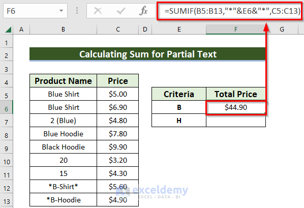
Method 2 – Calculating a Sum If a Cell Contains a Part of a Text String
Let’s sum up the price of products whose name contains a given text which is part of the whole name.
Steps:
- Insert the following formula in Cell F6.
=SUMIF(B5:B13,"*"&E6&"*",C5:C13)- Press Enter.
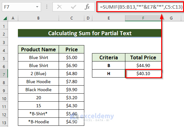
Here’s the formula in the cell below:
=SUMIF(B5:B13,"*"&E7&"*",C5:C13)You can observe that here the summation result is showing results for all the products that have an H in the name. It doesn’t matter whether H is at the start, in the middle, or at the end of the text.
How does the Formula Work:
Here, the first argument of the SUMIF formula is range. Here the range is B5:B13 where the condition is applied.
Next, in the criteria part of the argument, the specific text is given. Here we see two examples for two different partial texts- “B” and “H”. The asterisk is given at the start and end of the specific word. This is used to indicate zero or more characters.
Then, the last argument is the sum_range. Here the range is C5:C13 which takes the specific cells based on the specific text, to sum up with SUMIF function.
Read More: How to Add Specific Cells in Excel (5 Simple Ways)
Method 3 – Determining a Sum If a Cell Contains Numbers
Steps:
- Insert the following formula in the result cell:
=SUM(IFERROR(--LEFT(B5:B13,FIND(" ",B5:B13&" ")-1),""))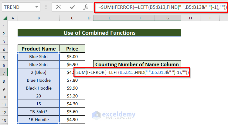
- Press Enter.
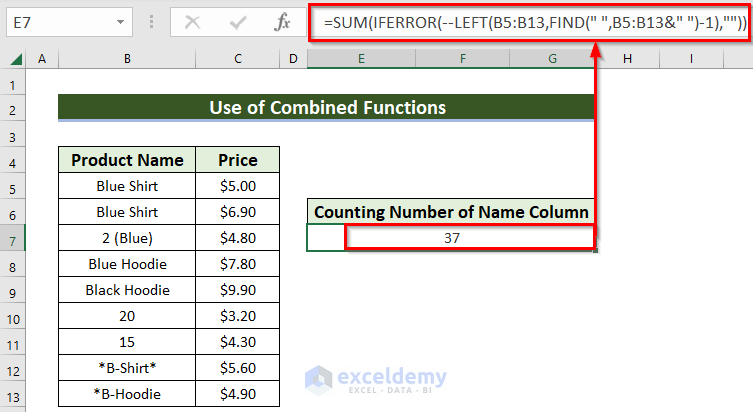
Formula Breakdown:
If we take the FIND formula:
FIND(" ",B5:B13&" ")-1It will find the number of characters in the texts and subtract it by 1. The resulting array will be:
{4;4;1;4;5;2;2;9;9}Next, if we look the LEFT formula with the FIND one:
LEFT(B5:B13,FIND(" ",B5:B13&" ")-1)It will show the numeric numbers only. Other values will show the #VALUE! error.
The result is:
{#VALUE!;#VALUE!;2;#VALUE!;#VALUE!;20;15;#VALUE!;#VALUE!}After that if we see the IFERROR array result for the formula
IFERROR(--LEFT(B5:B13,FIND(" ",B5:B13&" ")-1),"")This will show numeric values for true and for error it will show blank. The result is shown in the array format:
{"";"";2;"";"";20;15;"";""}Finally, the result of IFERROR is summed to get the result using the SUM formula, through which we will get the final result 37.
Read More: How to Add Numbers in Excel (2 Easy Ways)
Similar Readings
- Sum Formula Shortcuts in Excel (3 Quick Ways)
- How to Add Multiple Cells in Excel (6 Methods)
- Excel Sum Last 5 Values in Row (Formula + VBA Code)
- How to Add Rows in Excel with Formula (5 ways)
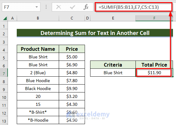
Method 4 – Computing a Sum If a Cell Contains Text Situated in Another Cell in Excel
Steps:
- Copy the following formula in Cell F7:
=SUMIF(B5:B13,E7,C5:C13)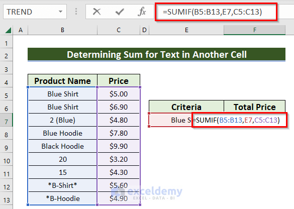
- Press Enter.
How Does the Formula Work:
Here, the first argument of the SUMIF formula is range. Here the range is B5:B13 where the condition is applied.
Next, in the criteria part of the argument, the text is given. Here we have “Blue Shirt” as the text in another cell.
Finally, the last argument is the sum_range. Here the range is C5:C13 which takes the specific cells based on the specific text, to sum up with SUMIF function.
Read More: Sum Cells in Excel: Continuous, Random, With Criteria, etc.
Method 5 – Finding a Sum If a Cell Contains an Asterisk
Steps:
- Insert the following formula in Cell E7:
=SUMIFS(C5:C13,B5:B13,"*~**")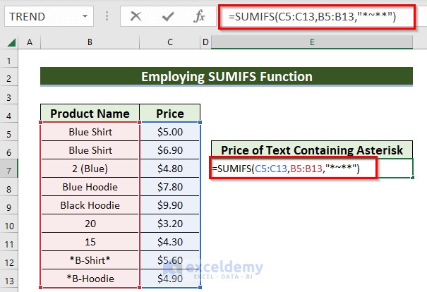
- Press Enter.
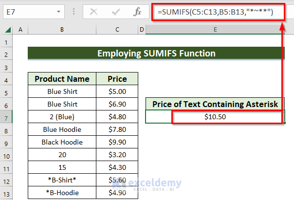
How Does the Formula Work:
Here, the first argument sum_range of the SUMIFS formula is the range of data from where we will get the result. In this case, the range is C5:C13.
Then, the criteria_range set is the second argument here. For this case, the range is B5:B13.
Lastly, the third argument is the set of criteria. We have an asterisk (*) as our criteria because we need to find texts with this sign. We can write this as ~*. Again, the asterisk is given at the start and end of the specific word. This indicates zero or more characters.
Read More: How to Sum Range of Cells in Row Using Excel VBA (6 Easy Methods)
Things to Remember
- Use a wildcard asterisk (*) at the start and end of the text to indicate zero or more other characters.
- Write any text or string within double quotes (
""). - The SUMIF function is not case sensitive while the FIND function is case-sensitive.
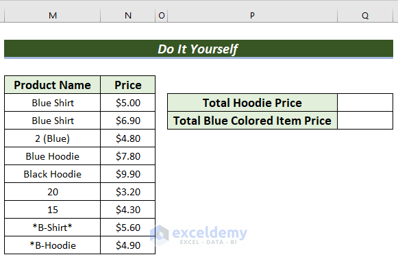
Practice Section
Now, you can practice by yourself.
Related articles
- How to Sum Multiple Rows and Columns in Excel
- Sum to End of a Column in Excel (8 Handy Methods)
- How to Sum Only Visible Cells in Excel (4 Quick Ways)
- [Fixed!] Excel SUM Formula Is Not Working and Returns 0 (3 Solutions)
- Shortcut for Sum in Excel (2 Quick Tricks)
- How to SUM with IF Condition in Excel (6 Suitable Examples)

