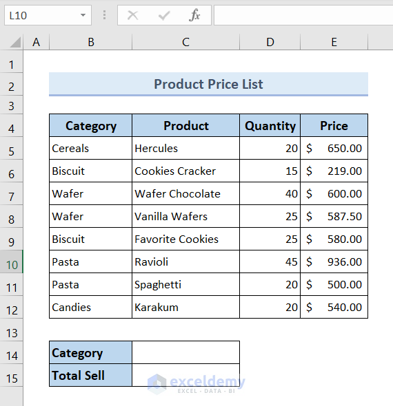
We will be using a sample product price list as a dataset to demonstrate all the methods throughout the article. Let’s have a sneak peek of it:
Method 1 – Using SUMIF Function to Sum If Cell Contains a Text in Excel
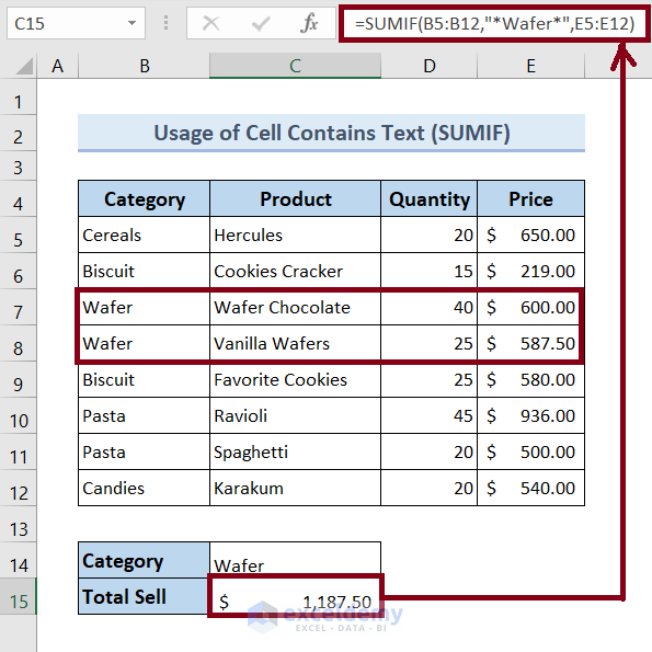
In the spreadsheet, we have a product price list with categories. So, in this section, we will try to calculate the total price of the products under the Wafer category.
Steps:
- Select cell C15.
- Put the following formula inside the cell:
=SUMIF(B5:B12,"*Wafer*", E5:E12)- Press Enter.
␥ Formula Breakdown:
Syntax: SUMIF(range, criteria, [sum_range])
- B5:B12 is the range where the SUMIF function will look for the word “Wafer”.
- “*Wafer*” the search keyword.
- E5: E12 is the sum range.
- =SUMIF(B5:B12,”*Wafer*”, E5:E12) returns the total price of the products under the “Wafer” category.
Method 2 – Applying Excel SUMIFS Function to Add Up Data If Cell Contains a Specific Text
Steps:
- Select cell C15.
- Input the following formula:
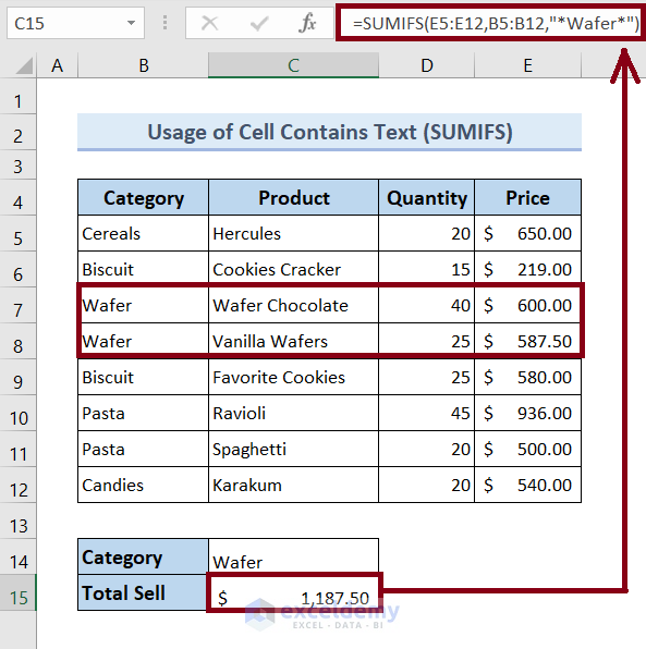
=SUMIFS(E5:E12,B5:B12,"*Wafer*")- Press Enter.
␥ Formula Breakdown:
Syntax: SUMIFS(sum_range, criteria_range1, criteria1, [criteria_range2, criteria2], …)
- E5: E12 is the sum range.
- B5:B12 is the range where the SUMIFS function will look for the word “Wafer”.
- “*Wafer*” is the search keyword.
- =SUMIFS(E5:E12, B5:B12,”*Wafer*”) returns the total price of the products under the “Wafer” category.
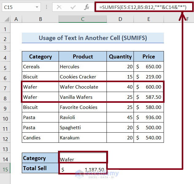
Method 3 – Applying SUMIF Function to Sum If Cell Contains Text in Another Cell in Excel
Steps:
- Create new cells to store the search terms and result.
- Select cell C15.
- Input the following formula.
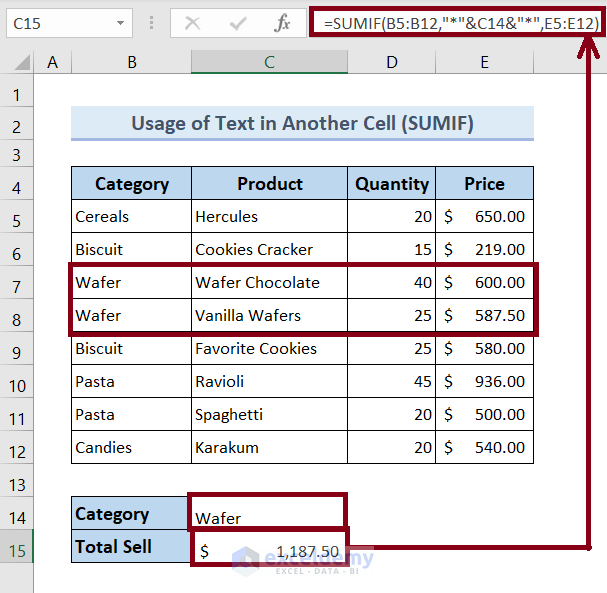
=SUMIF(B5:B12,"*"&C14&"*",E5:E12)- Press Enter.
␥ Formula Breakdown:
Syntax: SUMIF(range, criteria, [sum_range])
- B5:B12 is the range where the SUMIF function will look for the word “Wafer”.
- “*”&C14&”*” refers to the address of the cell that contains the search keyword “Wafer”.
- E5: E12 is the sum range.
- =SUMIF(B5:B12,”*”&C14&”*”,E5:E12) returns the total price of the products under the “Wafer” category.
Method 4 – Adding Up If Cell Contains Text in Another Cell Using SUMIFS Function
Steps:
- Select cell C15.
- Paste the following formula into it:
=SUMIFS(E5:E12,B5:B12,"*"&C14&"*")- Press Enter.
␥ Formula Breakdown:
Syntax: SUMIFS(sum_range, criteria_range1, criteria1, [criteria_range2, criteria2], …)
- E5: E12 is the sum range.
- B5:B12 is the range where the SUMIFS function will look for the word “Wafer”.
- “”*”&C14&”*”” refers to the address of the cell that contains the search keyword “Wafer”.
- =SUMIFS(E5:E12,B5:B12,”*”&C14&”*”) returns the total price of the products under the “Wafer” category.
Read More: How to Sum If Cell Contains Text in Another Cell in Excel
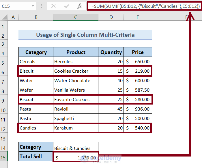
Method 5 – Calculating the Total Price Based on Multiple Text Type (AND Criteria)
Case 5.1 Summing If Cell Contains a Text Within a Single Column in Excel
This time, we will calculate the total price of the products under the Biscuit and Candies category.
Steps:
- Select cell C15.
- Type this formula:
=SUM(SUMIF(B5:B12, {"Biscuit","Candies"},E5:E12))- Hit Enter.
␥ Formula Breakdown:
Syntax of the SUM function: SUM(number1,[number2],…)
Syntax of the SUMIF function: SUMIF(range, criteria, [sum_range])
- B5:B12 is the range where the SUMIF function will look for the word “Wafer”.
- “Biscuit”,”Candies” are the search keywords.
- E5: E12 is the sum range.
- =SUM(SUMIF(B5:B12, {“Biscuit”,”Candies”},E5:E12)) returns the total price of the products under the Biscuit and Candies category.
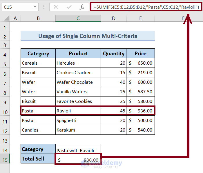
Case 5.2 Summing If Cell Contains Text Within Multiple Columns in Excel
Now we will try to calculate the total price of the products under the “Pasta” category and have the word “Ravioli” in their product name.
Steps:
- Go to cell C15.
- Input the following:
=SUMIFS(E5:E12,B5:B12,"Pasta",C5:C12,"Ravioli")- Press Enter.
␥ Formula Breakdown:
Syntax: SUMIFS(sum_range, criteria_range1, criteria1, [criteria_range2, criteria2], …)
- E5: E12 is the sum range.
- B5:B12 is the range where the SUMIFS function will look for the word “Pasta”.
- “Pasta”,”Ravioli” are the search keywords.
- C5:C12 is the range where the SUMIFS function will look for the word “Ravioli”.
- =SUMIFS(E5:E12,B5:B12,”Pasta”,C5:C12,”Ravioli”) returns the total price of the products under the “Pasta” category and have “Ravioli” in the product name.
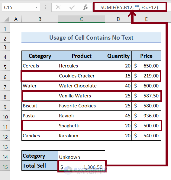
Method 6 – Calculating the Sum Value If the Cell Contains No Text in Excel
This time, we will calculate the total price for the products whose categories are missing.
Steps:
- Select cell C15.
- Input the following formula:
=SUMIF(B5:B12, "", E5:E12)- Press Enter.
␥ Formula Breakdown:
Syntax: SUMIF(range, criteria, [sum_range])
- B5:B12 is the range where the SUMIF function will look for the missing category.
- “” is specifies blank cell.
- E5: E12 is the sum range.
- =SUMIF(B5:B12, “”, E5:E12) returns the total price of the products whose categories are missing.
Read More: How to Sum Only Numbers and Ignore Text in Same Cell in Excel
Download Practice Workbook
You are recommended to download the Excel file and practice along with it.
Excel Sum If Cell Contains Text: Knowledge Hub
- How to Assign Value to Text and Sum in Excel
- How to Sum Text Values Like Numbers in Excel
- How to Sum Names in Excel
<< Go Back to Excel SUMIF Function | Excel Functions | Learn Excel
Get FREE Advanced Excel Exercises with Solutions!
