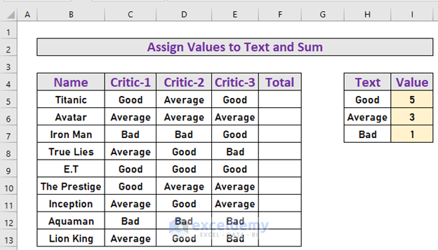
We have some movies and the remarks of some critics. We have assigned some values to these remarks. With these values, we will calculate the total score of each movie.
Method 1 – Merge SUM and COUNTIF Functions to Assign a Value to Text and Sum
Steps:
- Go to F5 and enter the following formula
=SUM(COUNTIF(C5:E5,$H$5:$H$7)*$I$5:$I$7)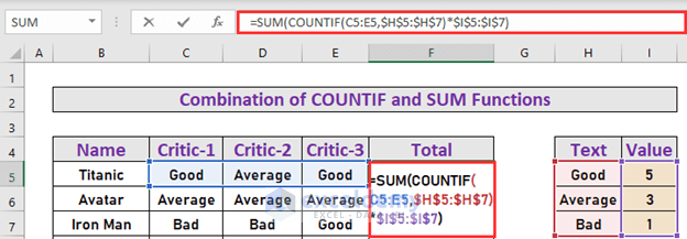
For each cell in C5:E5, the formula counts the instances of text in the lookup range, then multiplies that with the respective result.
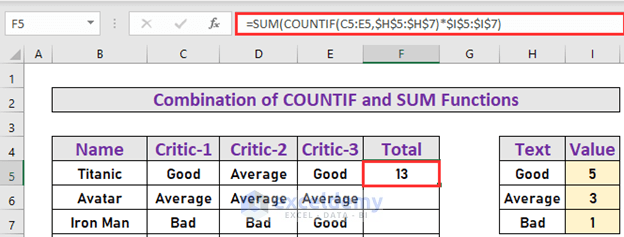
- Press Enter. Excel will return the output.
Note: This is an array formula. If you are using earlier versions of Excel, you must press Ctrl + Shift + Enter instead of Enter only.
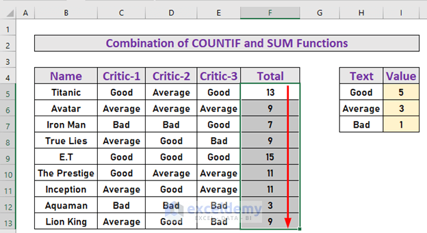
- Use the Fill Handle to AutoFill to F13.
Read More: How to Sum Text Values Like Numbers in Excel
Method 2 – Combine SUM, INDEX, MATCH, N, and IF Functions to Assign Value to Text and Sum
Steps:
- Go to F5 and insert the following formula:
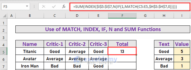
=SUM(INDEX($I$5:$I$7,N(IF(1,MATCH(C5:E5,$H$5:$H$7,0)))))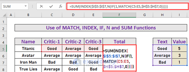
Formula Breakdown:
- MATCH(C5:E5,$H$5:$H$7,0)
- Output: {1,2,1}
- IF(1,MATCH(C5:E5,$H$5:$H$7,0))
- Output: {1,2,1}
- N(IF(1,MATCH(C5:E5,$H$5:$H$7,0)))
- Output: {1,2,1}
- INDEX($I$5:$I$7,N(IF(1,MATCH(C5:E5,$H$5:$H$7,0))))
- Output: {5,3,5}
- SUM(INDEX($I$5:$I$7,N(IF(1,MATCH(C5:E5,$H$5:$H$7,0)))))
- SUM(5,3,5)
- Output: 13
- Hit Enter.
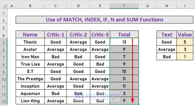
- Use the Fill Handle to AutoFill to F13.
Read More: How to Sum Only Numbers and Ignore Text in Same Cell in Excel
Download the Practice Workbook
Related Articles
<< Go Back to Excel Sum If Cell Contains Text | Excel SUMIF Function | Excel Functions | Learn Excel
Get FREE Advanced Excel Exercises with Solutions!

Very useful
Good job and God bless you
Hi G0DWIN,
Thank you for your kind words!