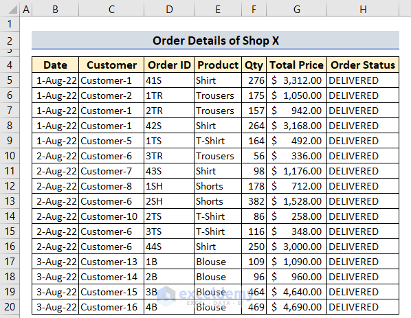
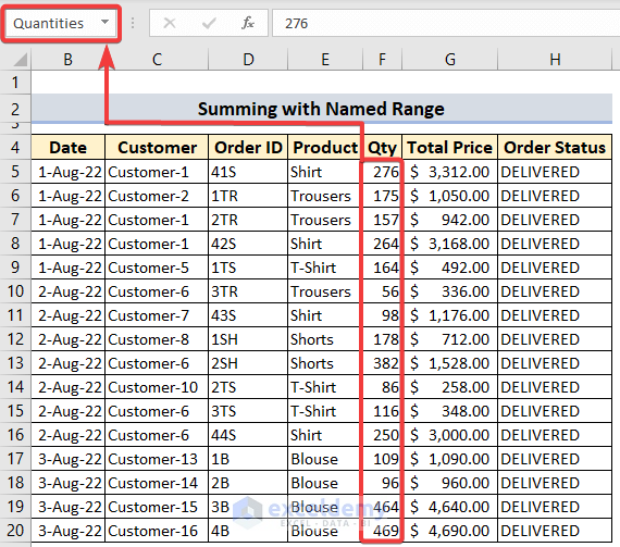
We’ll use the following dataset which contains order details. We’ll use the Product or Customer names to sum values.
Method 1 – Sum for One or Multiple Names Using Excel SUMIF or SUMIFS Functions
Steps:
- For the total quantity and total order prices for Customer-1, put the following formulas in cells J5 and K5.
Formula for Total Quantity:
=SUMIF(C5:C20, C5, F5:F20)Formula for Order Price:
=SUMIF(C5:C20, C5, G5:G20)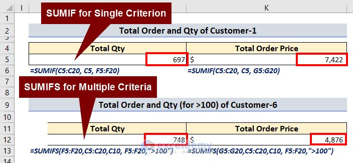
- We can apply the SUMIFS function to add more criteria. For the total order quantity and price for Customers only for those greater than 100 pieces, insert the following formula in cells J12 and K12.
Formula for Total Quantity (Which Are >100):
=SUMIFS(F5:F20,C5:C20,C10, F5:F20,">100")Formula for Total Price (Whose Quantity Are >100):
=SUMIFS(G5:G20,C5:C20,C10, F5:F20,">100")Note:
You could use “Customer-1” instead of C10 inside the formulas to set name criteria.
Read More: How to Sum If Cell Contains Text in Another Cell in Excel
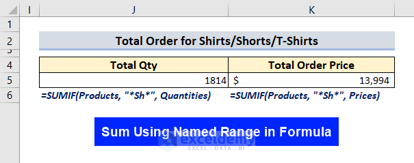
Method 2 – Sum Names for Partial Matches in Excel
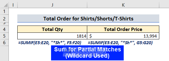
We have products such as shirts, t-shirts, and shorts. You see “sh” is common in these products’ names. We can set a formula using wildcard characters to get the total for all these products.
Steps:
- Go to cell J5 and insert the following formula.
=SUMIF(E5:E20, "*Sh*", F5:F20)- Hit the Enter button.
Read More: How to Assign Value to Text and Sum in Excel
Method 3 – Performing a Summation of a Named Range in Excel
Steps:
- Select the product column.
- Rename it as Products via the name text box on the ribbon (left to the formula bar). Use an underscore (_) if you want to use two or more words in the name box.
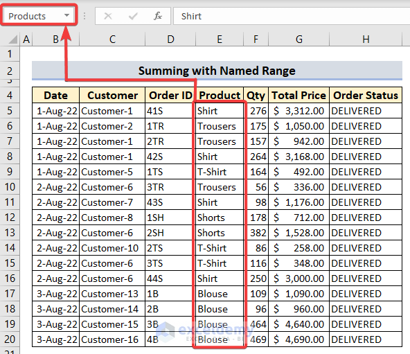
- Rename the Quantity Column as Quantities.
- Apply the following formula in cell J5.
=SUMIF(Products, "*Sh*", Quantities)We don’t have to use the range as a reference since we used named ranges.
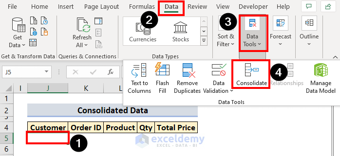
Method 4 – Using the Consolidate Option to Summarize the Total for Specified Names
We’ll combine the columns labeled Customer, Qty, and Total Price by consolidating.
Steps:
- Go to Consolidate under Data Tools under the Data tab.
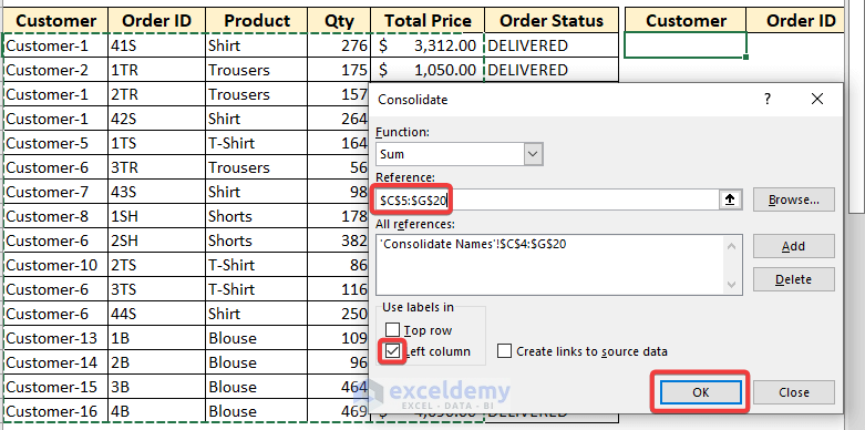
- A Consolidate pop-up will then show up here.
- Select Sum in the Function area.
- Select the data range you want to consolidate. Here it is C5:G20.
- Mark Left Column under Use Labels.
- Click OK.
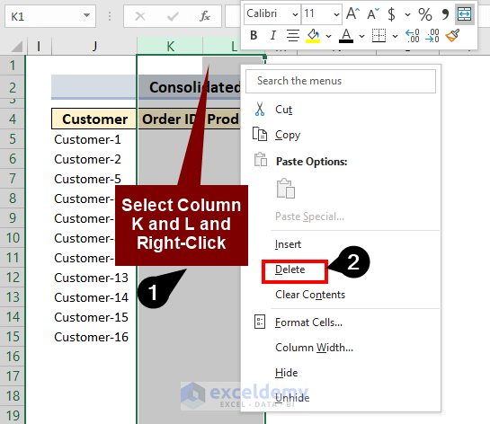
- We have some undesirable columns like the 2nd (K) and 3rd (L) column.
- Select the 2nd and 3rd columns, right-click, and select Delete.
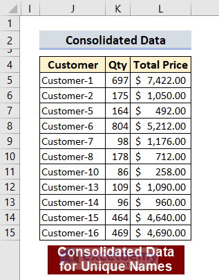
- Here is the final data.
Download the Practice Workbook
Related Articles
<< Go Back to Excel Sum If Cell Contains Text | Excel SUMIF Function | Excel Functions | Learn Excel
Get FREE Advanced Excel Exercises with Solutions!
