Download the Practice Workbook
5 Simple Methods to Sum Last 5 Values in a Row in Excel
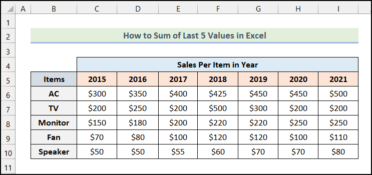
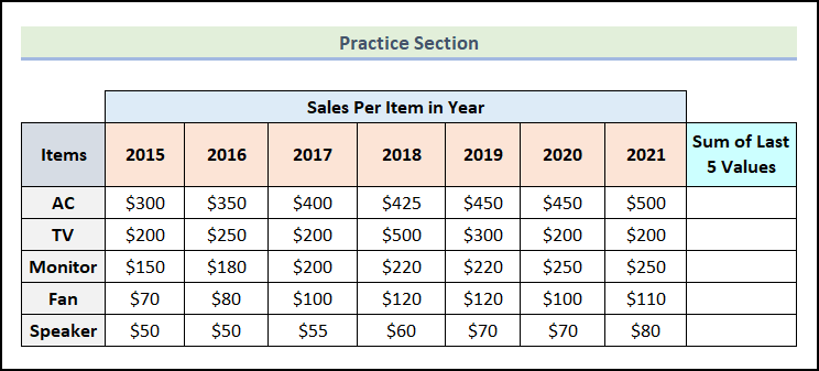
We have a dataset that contains the Sales of five items from 2015 to 2021. We have to find the sum of the sales from 2017 to 2021.
Method 1 – Using the OFFSET Function
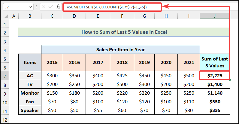
- Enter the following formula in cell J7.
=SUM(OFFSET($C7,0,COUNT($C7:$I7)-1,,-5))Here, C7 (the sales of AC in 2015) is the starting point, and the number of rows is 0 because the sales of AC over 7 years are in the cell of the starting point(C7).
Formula Breakdown
- The COUNT function is used in the formula to count the number of columns from the starting point.
- Output → 7.
- OFFSET($C7,0,COUNT($C7:$I7)-1,,-5) becomes OFFSET($C7,0,7-1,,-5).
- $C7 → It is the reference argument.
- 0 → This indicates the rows argument.
- 7-1 → This refers to the cols argument.
- -5 → It is the [width] argument.
- Output → {400,425,450,450,500}.
- The SUM function will return the sum of the specified values.
- SUM(OFFSET($C7,0,COUNT($C7:$I7)-1,,-5)) becomes SUM({400,425,450,450,500}).
- Output → $2,225.
Read More: How to Sum Multiple Rows and Columns in Excel
Method 2 – Utilizing INDEX and MATCH Functions
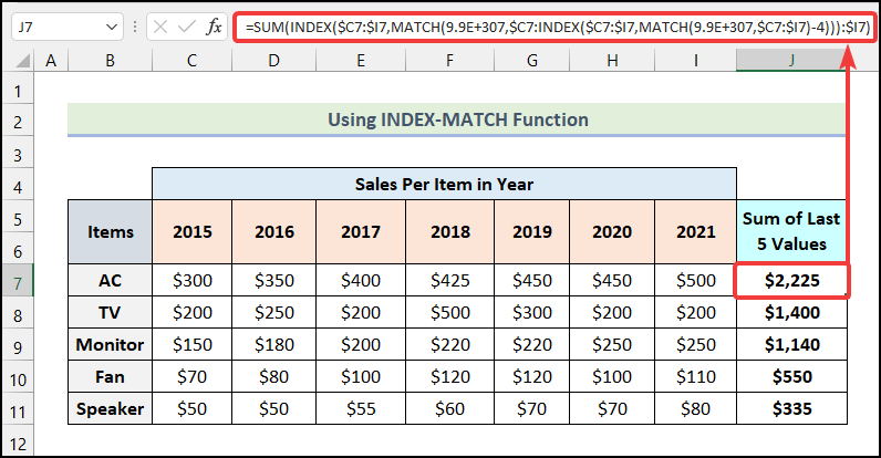
- Use the following formula in cell J7.
=SUM(INDEX($C7:$I7,MATCH(9.9E+307,$C7:INDEX($C7:$I7,MATCH(9.9E+307,$C7:$I7)-4))):$I7)In this formula, C7:I7 is the cell range for the sales of AC over years, C7 is the sales of AC in 2015, and I7 is the sales of AC in 2021.
9.9E+307 is an extremely huge number and it is used to find the greatest number that can be obtained by combining the other parts of the formula. -4 is used because we are finding the last 5 values.
Formula Breakdown
- The 1st MATCH function is MATCH(9.9E+307,$C7:$I7).
- 9.9E+307 → It is the lookup_value argument.
- $C7:$I7 → This represents the lookup_array argument.
- Output → 7.
- The 1st INDEX function, INDEX($C7:$I7,MATCH(9.9E+307,$C7:$I7)-4) becomes INDEX($C7:$I7,7-4).
- $C7:$I7 → It is the array argument.
- 7-4 → This indicates the row_num argument.
- Output → 400.
- The 2nd MATCH function is MATCH(9.9E+307,$C7:INDEX($C7:$I7,MATCH(9.9E+307,$C7:$I7)-4)) and it becomes MATCH(9.9E+307,$C7:400).
- Output → 3.
- The 2nd INDEX function, INDEX($C7:$I7,MATCH(9.9E+307,$C7:INDEX($C7:$I7,MATCH(9.9E+307,$C7:$I7)-4))) becomes INDEX($C7:$I7,3),
- Output → 400.
- SUM(INDEX($C7:$I7,MATCH(9.9E+307,$C7:INDEX($C7:$I7,MATCH(9.9E+307,$C7:$I7)-4))):$I7) becomes SUM(400:$I7)B.
- Output → $2,225.
Read More: How to Sum Range of Cells in Row Using Excel VBA (6 Easy Methods)
Method 3 – Applying LARGE and COLUMN Functions
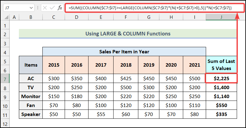
- Apply the following formula in cell J7.
=SUM((COLUMN($C7:$I7)>=LARGE(COLUMN($C7:$I7)*(N(+$C7:$I7)>0),5))*N(+$C7:$I7))C7:I7 is the cell range for the sales of AC over the years.
Formula Breakdown
- The N function is used to convert the cell value into a number.
- The COLUMN function here specifies the column number for the last 5 years’ sales.
- COLUMN($C7:$I7) is the 1st COLUMN function.
- $C7:$I7 → It is the [reference] argument.
- Output → {3,4,5,6,7,8,9}.
- LARGE(COLUMN($C7:$I7)*(N(+$C7:$I7)>0),5) becomes LARGE({3,4,5,6,7,8,9},5).
- Here, {3,4,5,6,7,8,9} → This indicates the array argument.
- 6 → It is the k argument.
- Output → 5.
- The 2nd COLUMN function COLUMN($C7:$I7) returns {3,4,5,6,7,8,9} as Output.
- (COLUMN($C7:$I7)>=LARGE(COLUMN($C7:$I7)*(N(+$C7:$I7)>0),5))*N(+$C7:$I7) becomes ({3,4,5,6,7,8,9}>=5)*{300,350,400,425,450,450,500}.
- Output → {0,0,400,425,450,450,500}.
- SUM((COLUMN($C7:$I7)>=LARGE(COLUMN($C7:$I7)*(N(+$C7:$I7)>0),5))*N(+$C7:$I7)) becomes SUM({0,0,400,425,450,450,500}).
- Output → $2,225.
Read More: All the Easy Ways to Add up (Sum) a column in Excel
Similar Readings
- How to Add Rows in Excel with Formula (5 ways)
- 3 Easy Ways to Sum Top n Values in Excel
- How to Sum Filtered Cells in Excel (5 Suitable Ways)
- Sum Cells in Excel: Continuous, Random, With Criteria, etc.
- How to Sum Selected Cells in Excel (4 Easy Methods)
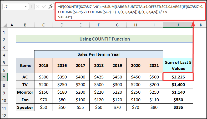
Method 4 – Using the COUNTIF Function
- Apply the following formula in cell J7.
=IF(COUNTIF($C7:$I7,">0")>=5,SUM(LARGE(SUBTOTAL(9,OFFSET($C7,0,LARGE(IF($C7:$I7>0,COLUMN($C7:$I7)-COLUMN($C7)+1)-1,{1,2,3,4,5}))),{1,2,3,4,5})),"< 5 Values")C7:I7 is the cell range for the sales of AC over years, C7 is the sales of AC in 2015.
Formula Breakdown
- The 1st IF function IF($C7:$I7>0,COLUMN($C7:$I7)-COLUMN($C7)+1).
- $C7:$I7>0 → It is the logical_test function.
- COLUMN($C7:$I7)-COLUMN($C7)+1 → This indicates the [value_if_true] argument.
- Output → {1,2,3,4,5,6,7}.
- LARGE(IF($C7:$I7>0,COLUMN($C7:$I7)-COLUMN($C7)+1)-1,{1,2,3,4,5}) becomes LARGE({1,2,3,4,5,6,7}-1,{1,2,3,4,5}).
- Output → {6,5,4,3,2}.
- The OFFSET function, OFFSET($C7,0,LARGE(IF($C7:$I7>0,COLUMN($C7:$I7)-COLUMN($C7)+1)-1,{1,2,3,4,5})) becomes OFFSET($C7,0,{6,5,4,3,2}).
- $C7 → It is the reference argument.
- 0 → This represents the rows argument.
- {6,5,4,3,2} → It indicates the cols argument.
- Output → {500,450,450,425,400}.
- SUBTOTAL(9,OFFSET($C7,0,LARGE(IF($C7:$I7>0,COLUMN($C7:$I7)-COLUMN($C7)+1)-1,{1,2,3,4,5}))) becomes SUBTOTAL(9,{500,450,450,425,400}).
- 9 → It refers to the function_num argument.
- {500,450,450,425,400} → This indicates the ref1 argument.
- Output → {500,450,450,425,400}.
- LARGE(SUBTOTAL(9,OFFSET($C7,0,LARGE(IF($C7:$I7>0,COLUMN($C7:$I7)-COLUMN($C7)+1)-1,{1,2,3,4,5}))),{1,2,3,4,5}) becomes LARGE({500,450,450,425,400},{1,2,3,4,5}).
- Output → {500,450,450,425,400}.
- SUM(LARGE(SUBTOTAL(9,OFFSET($C7,0,LARGE(IF($C7:$I7>0,COLUMN($C7:$I7)-COLUMN($C7)+1)-1,{1,2,3,4,5}))),{1,2,3,4,5})) becomes SUM({500,450,450,425,400}).
- Output → 2225.
- COUNTIF($C7:$I7,”>0″) returns 7 as output.
- IF(COUNTIF($C7:$I7,”>0″)>=5,SUM(LARGE(SUBTOTAL(9,OFFSET($C7,0,LARGE(IF($C7:$I7>0,COLUMN($C7:$I7)-COLUMN($C7)+1)-1,{1,2,3,4,5}))),{1,2,3,4,5})),”< 5 Values”) becomes IF(7>=5,2225,”< 5 Values”).
- 7>=5 → It is the logical_test argument.
- 2225 → It indicates the [value_if_true] argument.
- “< 5 Values” → This refers to the [value_if_false] argument.
- Output → $2,225.
Read More: How to Sum Cells with Text and Numbers in Excel (2 Easy Ways)
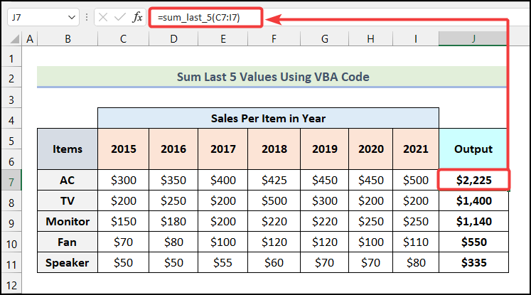
Method 5 – Using VBA Code
- Go to Developer and select Visual Basic.
- Click on Insert and select Module.
- Insert the following code for finding the sum of the last 5 sales for AC items.
Function sum_last_5(input_cells As Range, _
Optional ByVal l_count As Long = 5) As Double
Dim x As Long, y As Long, sum As Double
On Error GoTo err_hdl
x = input_cells.Count
Do While l_count > 0
If input_cells(x) <> "" Then
sum = sum + input_cells(x)
l_count = l_count - 1
End If
x = x - 1
Loop
function_exit: sum_last_5 = sum
Exit Function
err_hdl: Resume function_exit
End Function
Code Breakdown
- We initiated function named sum_last_5.
- Inside the function arguments, we declared a variable input_cell as Range.
- We assigned the output data type of the function as Double.
- We declared 3 variables.
- We used an On Error statement to enable an error-handling routine.
- We assigned the Count of input_cells in variable x.
- We initiated a Do While loop.
- We used an IF statement to check whether the input_cells are blank or not.
- We added the input_cells variable with the sum variable and again assigned it back to the sum variable.
- We subtracted 1 from the l_count variable and again assigned it back to the l_count variable.
- We ended the IF statement.
- We subtracted 1 from the variable x and again assigned it back to the variable x.
- We closed the Do While loop.
- We specified the exit conditions for the function.
- Save the file as an .xlsm.
- Use the formula given below in cell J7.
=sum_last_5(C7:I7)You will have the following outputs.
Read More: How to Add Multiple Cells in Excel (6 Methods)
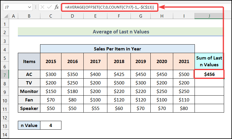
How to Average Last N Values in a Row in Excel
We’ll calculate the Average of the last 4 values in a row.
Steps:
- Use the following formula in cell J7.
=AVERAGE(OFFSET(C7,0,COUNT(C7:I7)-1,,-$C$13))- Press Enter.
Formula Breakdown
- The COUNT function, COUNT(C7:I7) returns 7 as output.
- OFFSET(C7,0,COUNT(C7:I7)-1,,-$C$13) becomes OFFSET(C7,0,7-1,,-$C$13).
- Output → {425,450,450,500}.
- The AVERAGE function will return the average of the specified numbers.
- AVERAGE(OFFSET(C7,0,COUNT(C7:I7)-1,,-$C$13)) becomes AVERAGE({425,450,450,500}).
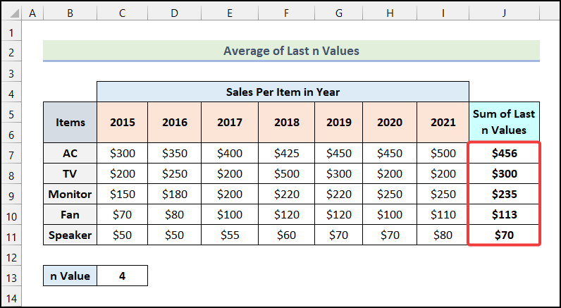
- Output → $456.
- Use the AutoFill option of Excel to get the remaining outputs as demonstrated in the following image.
How to Sum Every 3 Cells in Excel
We have the monthly sales data for different Items for a store. We’ll calculate the Quarterly Sales of the Items.
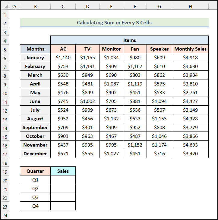
Steps:
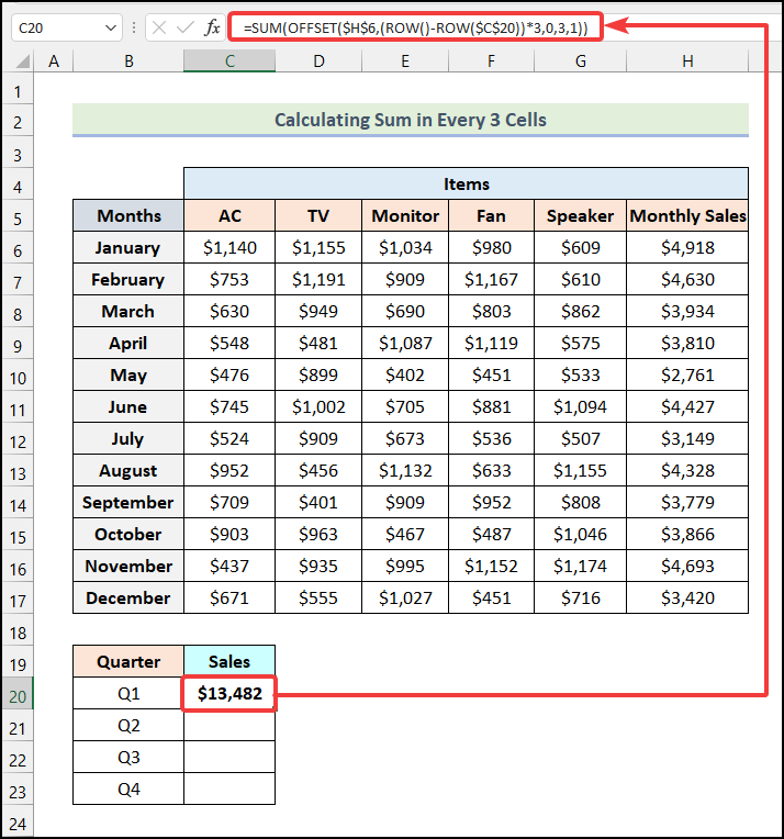
- Use the following formula in cell C20.
=SUM(OFFSET($H$6,(ROW()-ROW($C$20))*3,0,3,1))Cell H6 is the Monthly Sales for the month of January, and cell C20 indicates the cell of Q1 Sales:
Formula Breakdown
- The ROW function, ROW($C$20) returns {20} as output.
- OFFSET($H$6,(ROW()-ROW($C$20))*3,0,3,1) becomes OFFSET($H$6,({20}-{20})*3,0,3,1).
- The SUM function will return the sum of the 3 cells.
- Output → $13,482.
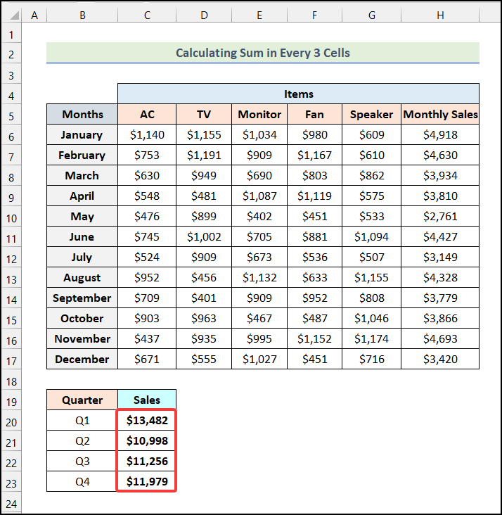
- Use the AutoFill feature of Excel to get the rest of the Quarterly Sales values.
Practice Section
In the Excel Workbook, we have provided a Practice Section on the right side of the worksheet.
Further Readings
- Shortcut for Sum in Excel (2 Quick Tricks)
- How to Sum Colored Cells in Excel (4 Ways)
- [Fixed!] Excel SUM Formula Is Not Working and Returns 0 (3 Solutions)
- Sum All Matches with VLOOKUP in Excel (3 Easy Ways)
- Excel Sum If a Cell Contains Criteria (5 Examples)

