Download Practice Workbook
5 Ways to Calculate Percentage of Marks in Excel
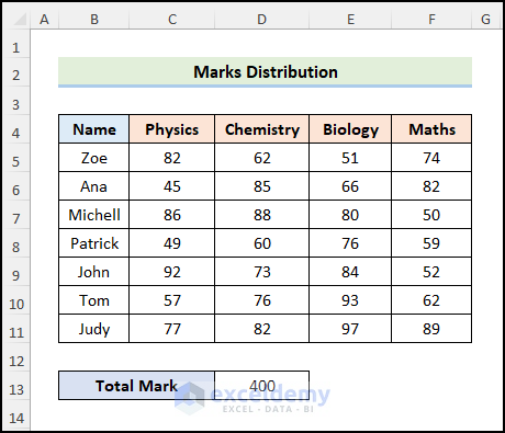
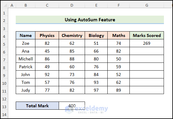
Our sample dataset contains student Names their scores in Physics, Chemistry, Biology, and Math.
Method 1 – Using Arithmetic Formula to Calculate Percentage of Marks
Steps:
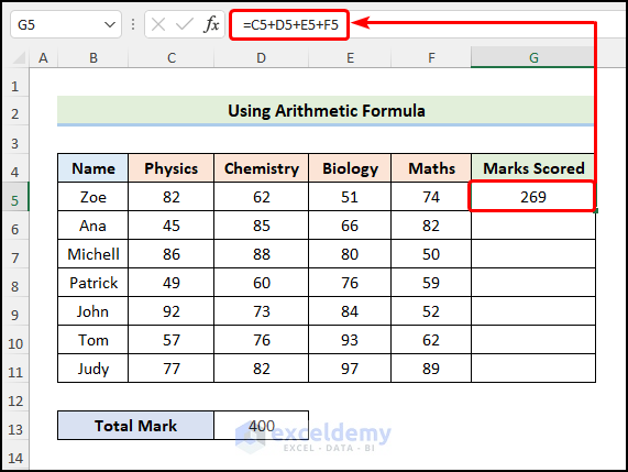
- Enter the following formula in G5.
=C5+D5+E5+F5
C5, D5, E5, and F5 indicate the marks obtained by Zoe in Physics, Chemistry, Biology, and Math, respectively.
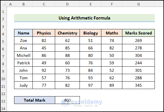
- Copy the formula to the cells below using the Fill Handle Tool.
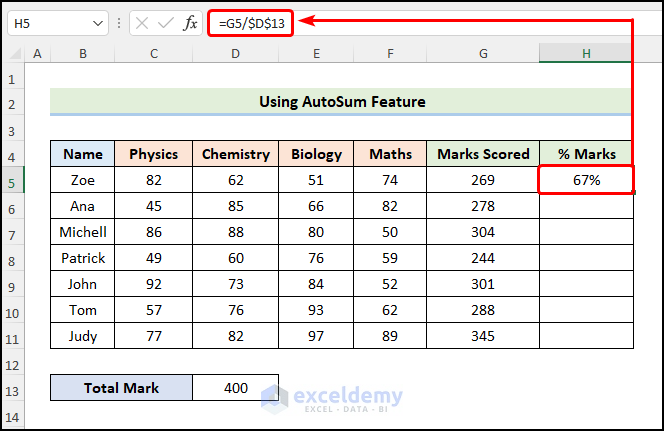
- Enter the following formula in H5.
=G5/$D$13
In this formula, the G5 cell refers to the Marks Scored while the D13 cell points to the Total Mark of 400.
Note: Please make sure to use Absolute Cell Reference by pressing the F4 key on your keyboard.
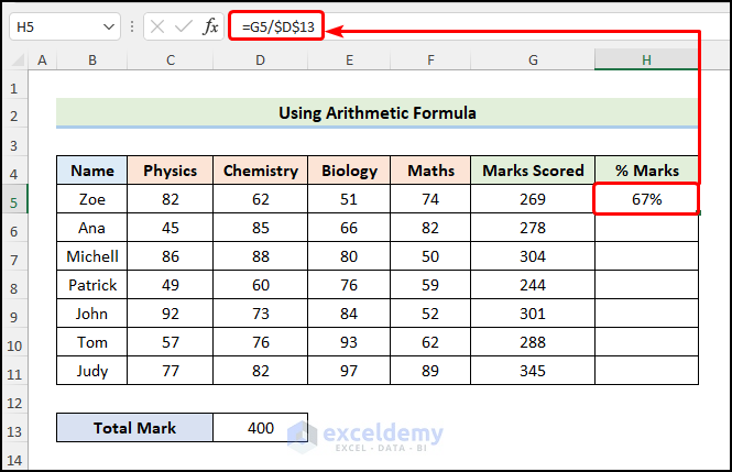
- Press CTRL + SHIFT + % on your keyboard to change the number format to percentage. Your result will look like the image below.

Read More: How to Apply Percentage Formula in Excel for Marksheet (7 Applications)
Method 2 – Calculating Percentage of Marks with SUM Function
Steps:
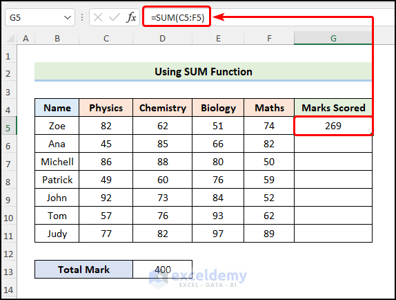
- Enter the following formula in G5.
=SUM(C5:F5)
C5:F5 range of cells points to the marks obtained by Zoe in the 4 subjects respectively.
- Enter the following formula in H5.
=G5/$D$13
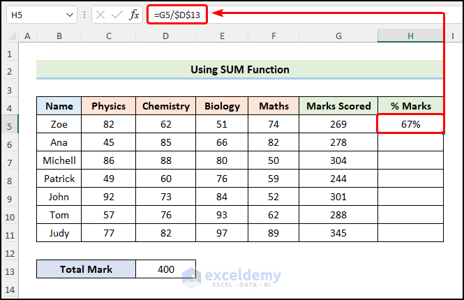
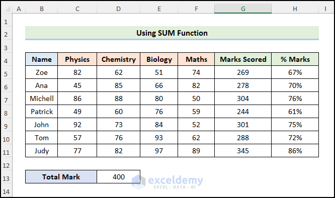
Your output will be displayed as shown in the following image.
Read More: Calculate Grade Using IF function in Excel (with Easy Steps)
Similar Readings
- Excel Formula for Pass or Fail with Color (5 Suitable Examples)
- How to Calculate Letter Grades in Excel (6 Simple Ways)
- How to Calculate Average Percentage of Marks in Excel (Top 4 Methods)
Method 3 – Utilizing AutoSum Feature to Calculate Percentage of Marks
Steps:
- Select the C5:F5 range of cells >> in the Editing section, click the AutoSum
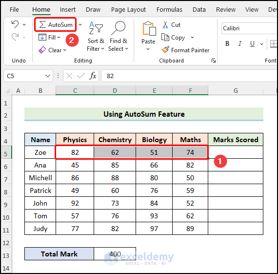
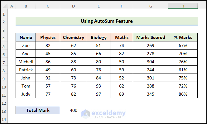
The result will be as shown below.
- Enter the following formula in the cell H5.
=G5/$D$13
The percentage will be displayed as shown in the image below.
Read More: How to Make a Grade Calculator in Excel (2 Suitable Ways)
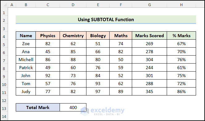
Method 4 – Applying the SUBTOTAL Function to Calculate Percentage of Marks
Steps:
- Enter the following formula in G5
=SUBTOTAL(109,C5:F5)
In the above formula, 109 (function_num argument) refers to the SUM function and the C5:F5 (ref1 argument) range of cells indicates the marks scored by Zoe in the 4 subjects.

- Enter the following formula in H5.
=G5/$D$13
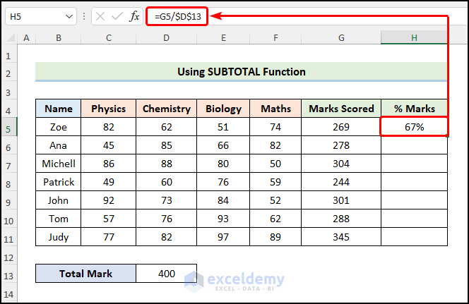
You will get the following subtotal.
Read More: How to Calculate Grade Percentage in Excel (3 Easy Ways)
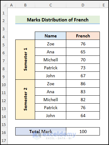
Method 5 – Employing the SUMIF Function to Calculate Percentage of Marks
To calculate the percentage of marks for a specific student from a given dataset, we can use the SUMIF function.
Let’s consider the Marks Distribution of French dataset in the B4:D14 cells. In this dataset, we have the student Names and their scores in French for two semesters.
Steps:
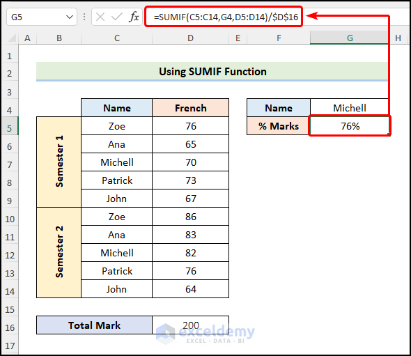
- Enter the following formula in the G5
=SUMIF(C5:C14,G4,D5:D14)/$D$16
The C5:C14 and the D5:D14 range of cells refer to the Name and the French columns respectively. In contrast, the G4 and the D16 cells point to the Name Michell and the Total Mark of 200.
Note: Please make sure to use Absolute Cell Reference by pressing the F4 key on your keyboard.
⚡ Formula Breakdown:
- =SUMIF(C5:C14,G4,D5:D14) → adds the cells specified by a given criteria or condition. C5:C14 is the range argument that refers to the Name G4 represents the criteria argument to apply within the given range. D5:D14 is the optional sum_range argument which indicates the values to sum within the range.
- Output → 152
- =SUMIF(C5:C14,G4,D5:D14)/$D$16 → becomes
- =152/$D$16 → In this expression, the value 152 is divided by the D16 cell which is the Total Mark of 200.
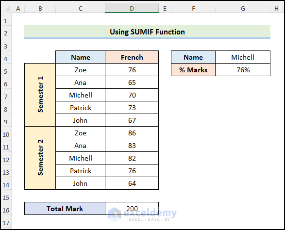
- 152/200 → 76%
Your output should look like the image shown below.
Read More: How to Make Result Sheet in Excel (with Easy Steps)
Related Articles
- How to Calculate Subject Wise Pass or Fail with Formula in Excel
- Make Automatic Marksheet in Excel (with Easy Steps)
- How to Compute Grades in Excel (3 Suitable Ways)
- Calculate Grades with Weighted Percentages in Excel

