Most of the time for educational purposes, you may need to use Excel Formula for Pass or Fail with Color. In this article, I will demonstrate how to use Excel Formula for Pass or Fail with Color.
5 Examples to Use Excel Formula for Pass or Fail with Color
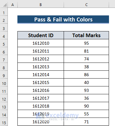
Here, I’m going to explain 5 methods of how to use Excel Formula for Pass or Fail with Color. For your better understanding, I will use a sample dataset. Which has 2 Columns. Those are Student ID and Total Marks. The sample dataset is given below.
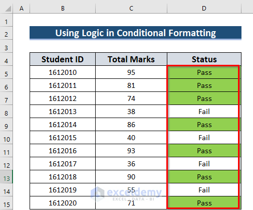
1. Using Logic in Conditional Formatting for Pass or Fail with Color
You can use the IF function for the Status of Pass or Fail. Furthermore, you can use Logical Test in Conditional Formatting as Excel Formula for Color the Pass or Fail status. The steps are given below.
Steps:
- Firstly, you have to select a different cell D5 where you want to see the Status.
- Secondly, you should use the corresponding formula in the D5 cell.
=IF(C5>=60,"Pass","Fail")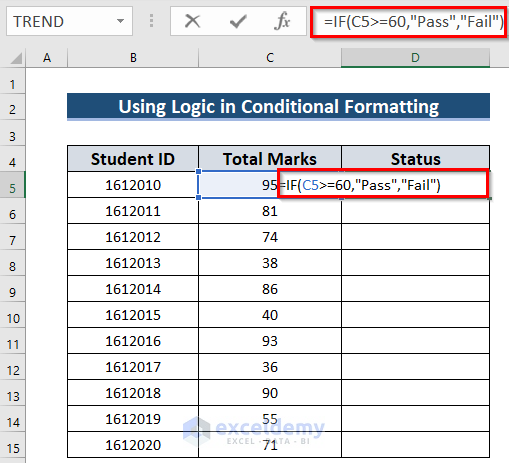
Formula Breakdown
Here, the IF function returns the result which will fulfill a given condition.
- Firstly, the C5>=60 denotes a logical test. Where the function will test that either the Total Marks is greater than or equal to 60.
- Secondly, “Pass” denotes that if the logic is TRUE on C5 then it will give Pass. Here, when you use any string then you must use the Inverted Comma.
- Finally, “Fail” denotes that if the logic is FALSE on C5 then it will give Fail.
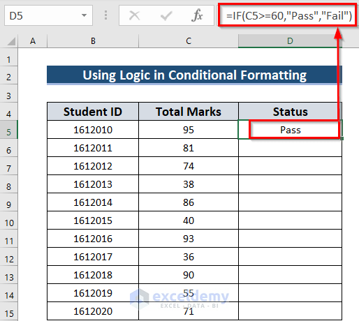
- Subsequently, you must press ENTER to get the result.
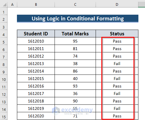
- After that, you have to drag the Fill Handle icon to AutoFill the corresponding data in the rest of the cells D6:D15. Or you can double-click on the Fill Handle

Finally, you will see the following result.
At this time, I will apply Conditional Formatting with the formula. Here, I will use a logical test.
- Firstly, you should select the data up to which you want to apply the Conditional Formatting to color the status Pass/Fail. Here, I have selected the data range D5:D15.
- Secondly, from the Home tab >> you must go to the Conditional Formatting command.
- Thirdly, you need to choose the New Rule option to apply the formula.

At this time, a dialog box named New Formatting Rule will appear.
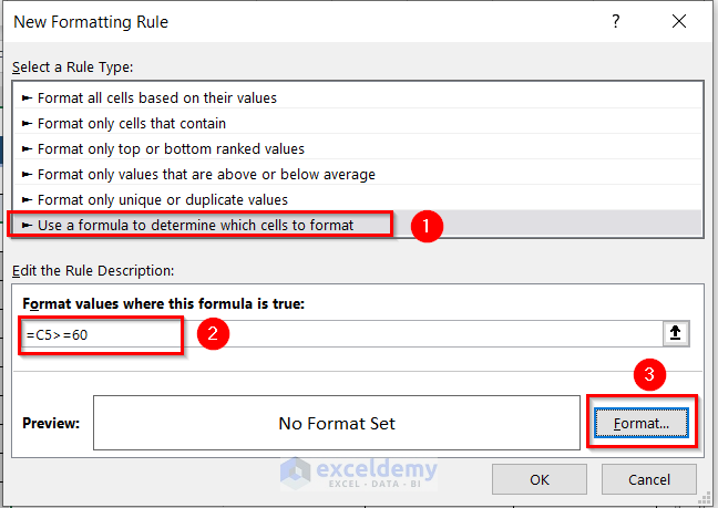
- Now, from that dialog box >> you have to select Use a formula to determine which cells to format.
- Then, you need to write down the following formula in the Format values where this formula is true:
=C5>=60Here, the Logical Test says that either the value of the C5 cell is greater than or equal to 60 otherwise less than 60. Also, if the value of C5 cell is greater than or equal to 60 then it will color the corresponding cell otherwise it remains with No color.
- After that, go to the Format menu.
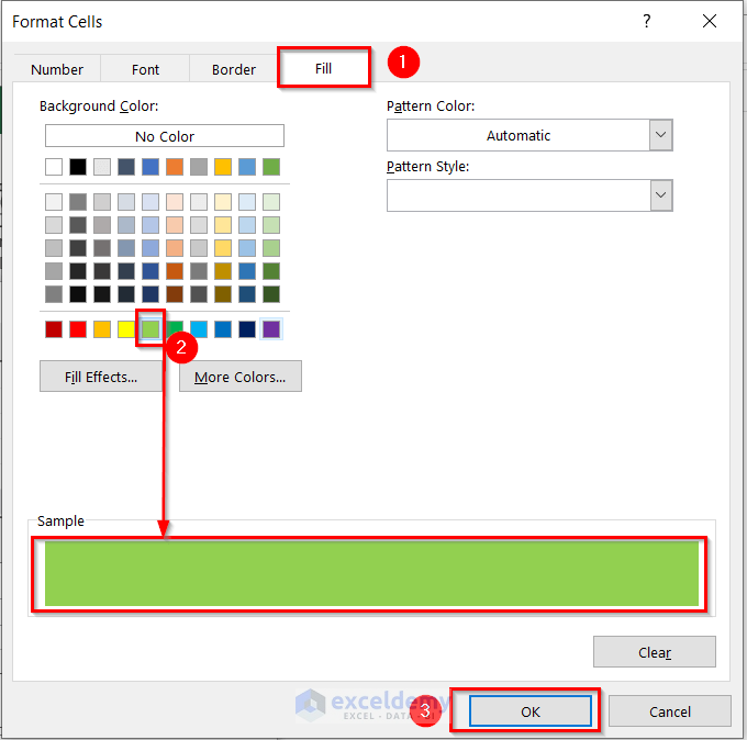
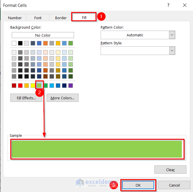
At this time, a dialog box named Format Cells will appear.
- Now, from the Fill option >> you have to choose any of the colors. Here, I have chosen Light Green. Also, you can see the sample In this case, try to choose any light color. Because the dark color may hide the inputted data. Then, you may need to change the Font Color.
- Then, you must press OK to apply the formation.
- After that, you have to press OK on the New Formatting Rule dialog box. Here, you can see the sample instantly in the Preview box.
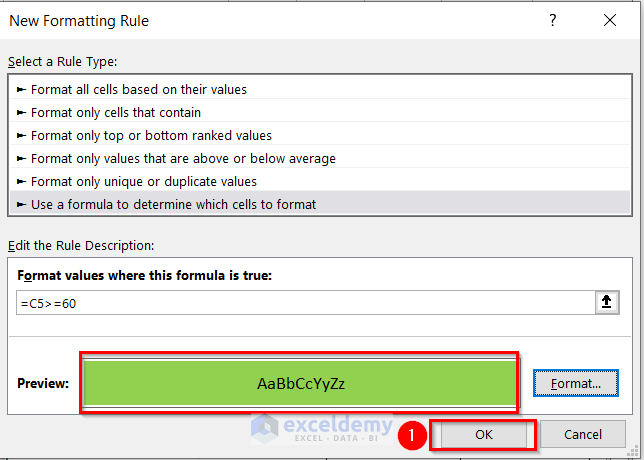
Finally, you will get the status “Pass” with color.
Similarly, you have to follow the same steps again to color the status “Fail”. Hence, I will apply the Conditional Formatting with the formula again. Here, I will use exactly the opposite logical test.
- Firstly, you should select the data up to which you want to apply the Conditional Formatting to color the status Pass/Fail. Here, I have selected the data range D5:D15.
- Secondly, from the Home tab >> you must go to the Conditional Formatting command.
- Thirdly, you need to choose the New Rule option to apply the formula.

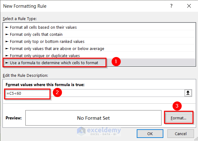
At this time, a dialog box named New Formatting Rule will appear.
- Now, from that dialog box >> you have to select Use a formula to determine which cells to format.
- Then, you need to write down the following formula in the Format values where this formula is true:
=C5<60Here, the Logical Test says that either the value of C5 cell is less than 60 or else. Also, if the value of C5 cell is less than 60 then it will color the corresponding cell otherwise it remains with No color.
- After that, go to the Format menu.
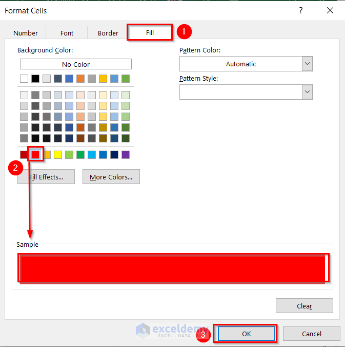
At this time, a dialog box named Format Cells will appear.
- Now, from the Fill option >> you have to choose any of the colors. Here, I have chosen Red. Also, you can see the sample In this case, try to choose any light color. Because, the dark color may hide the inputted data. Then, you may need to change the Font Color.
- Then, you must press OK to apply the formation.
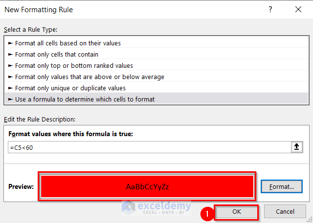
- After that, you have to press OK on the New Formatting Rule dialog box. Here, you can see the sample instantly in the Preview box.
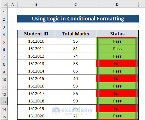
Finally, you will get both the status “Pass or Fail” with colors.
Read More: How to Calculate Subject Wise Pass or Fail with Formula in Excel
2. Use of IF Function and Text That Contains Feature
You can use the IF function for the Status of Pass or Fail. Furthermore, you can use the Text That Contains feature in Conditional Formatting as Excel Formula for Color the Pass or Fail status. The steps are given below.
Steps:
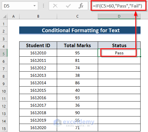
- Firstly, you have to select a different cell D5 where you want to see the Status.
- Secondly, you should use the corresponding formula in the D5
=IF(C5>60,"Pass","Fail")- Subsequently, you must press ENTER to get the result.
Formula Breakdown
Here, the IF function returns the result which will fulfill a given condition.
- Firstly, the C5>60 denotes a logical test. Where the function will test that either the Total Marks is greater than 60.
- Secondly, “Pass” denotes that if the logic is TRUE on C5 then it will give Pass. Here, when you use any string then you must use the Inverted Comma.
- Finally, “Fail” denotes that if the logic is FALSE on C5 then it will give Fail.
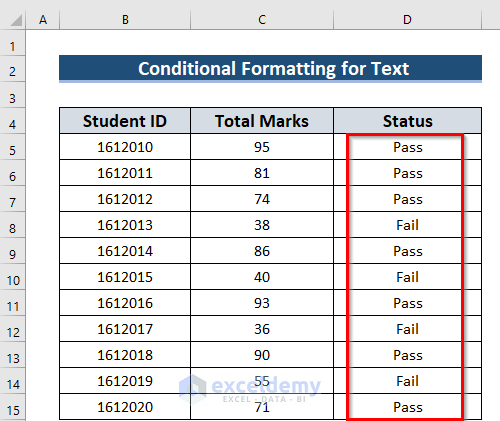
- After that, you can double-click on the Fill Handle icon to AutoFill the corresponding data in the rest of the cells D6:D15. .
Finally, you will get the Status.
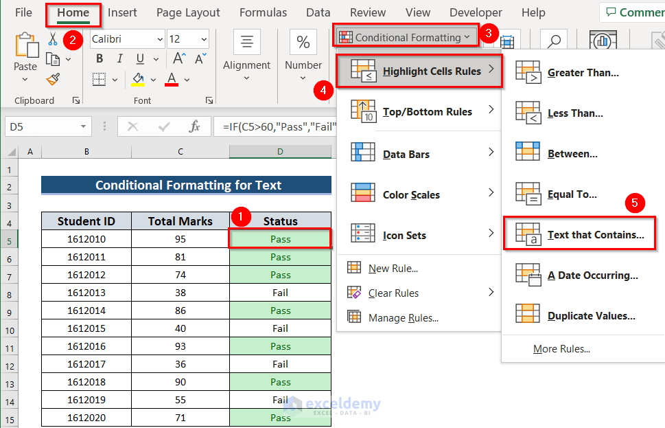
At this time, I will apply the Conditional Formatting to color the status.
- Firstly, you should select the data at which you want to apply the Conditional Formatting to color the status Pass/Fail. Here, I have selected the D5 cell.
- Secondly, from the Home tab >> you must go to the Conditional Formatting command.
- Thirdly, you need to choose the Text that Contains feature.

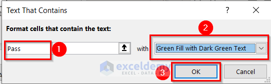
At this time a dialog box named Text That Contains will appear.
- Now, write down the target text “Pass” in the Format cells that contain the text box.
- Then, select the preferred color from the drop-down arrow.
- Finally, press OK to get the changes.
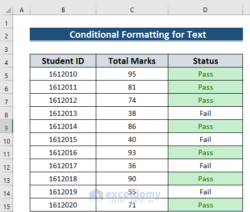
- After that, you can double-click on the Fill Handle icon to AutoFill the corresponding data in the rest of the cells D6:D15.

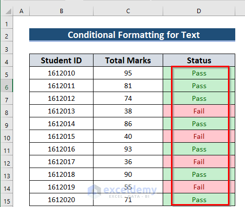
Finally, you will get the colored Status.
Similarly, you have to follow the same steps again to color the status “Fail”.
- Firstly, you should select the data at which you want to apply Conditional Formatting to color the status Pass/Fail. Here, I have selected the data range D5.
- Secondly, from the Home tab >> you must go to the Conditional Formatting command.
- Thirdly, you need to choose the Text that Contains the feature.
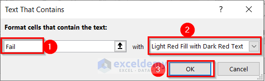
At this time a dialog box named Text That Contains will appear.
- Now, write down the target text “Fail” in the Format cells that contain the text box.
- Then, select the preferred color from the drop-down arrow.
- Finally, press OK to get the changes.
- After that, you can double click on the Fill Handle icon to AutoFill the corresponding data in the rest of the cells D6:D15.

Lastly, you will see the colored Pass/Fail.
Read More: How to Make Automatic Marksheet in Excel
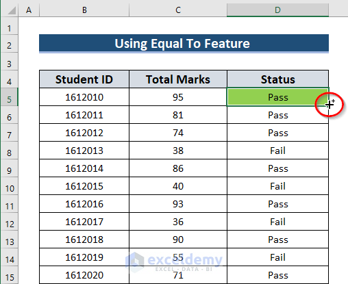
3. Applying Equal To Feature as Excel Formula for Pass or Fail with Color
You can use the IF function for the Status of Pass or Fail. Furthermore, you can use the Equal To feature in Conditional Formatting as Excel Formula for Color the Pass or Fail status.
- Now, you can follow method-1 to make the Status either Pass or Fail.

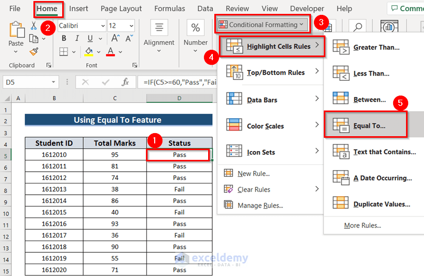
- Now, you should select the data at which you want to apply the Conditional Formatting to color the status Pass/Fail. Here, I have selected the D5 cell.
- Then, from the Home tab >> you must go to the Conditional Formatting command.
- After that, you need to choose the Equal To feature.
At this time a dialog box named Equal To will appear.
- Now, write down the target text “Pass” in the Format cells that are EQUAL TO box.
- Then, select the preferred color from the drop-down arrow. Here, I selected Custom Format.

At this time, a dialog box named Format Cells will appear.
- Now, from the Fill option >> you have to choose any of the colors. Here, I have chosen Light Green. Also, you can see the sample In this case, try to choose any light color. Because the dark color may hide the inputted data. Then, you may need to change the Font Color.
- Then, you must press OK to apply the formation.
Subsequently, the dialog box named Equal To will appear again.
- At this time, press OK on the Equal To dialog box to get the changes.

Similarly, you have to follow the same steps again to color the status “Fail”.
- Firstly, you should select the data at which you want to apply the Conditional Formatting to color the status Pass/Fail. Here, I have selected the data range D5.
- Secondly, from the Home tab >> you must go to the Conditional Formatting command.
- Thirdly, you need to choose the Equal To feature.

At this time a dialog box named Equal To will appear.
- Now, write down the target text “Fail” in the Format cells that are EQUAL TO box.
- Then, select the preferred color from the drop down arrow.
- Lastly, press Ok.

- After that, you can double click on the Fill Handle icon to AutoFill the corresponding data in the rest of the cells D6:D15.
At last, you will see the colored Pass/Fail.

Read More: How to Compute Grades in Excel
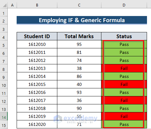
4. Employing IF Function and Generic Formula in Conditional Formatting
You can employ the IF function for the Status of Pass or Fail. Furthermore, you can use the Generic formula in Conditional Formatting as Excel Formula for Color the Pass or Fail status. The steps are given below.
Steps:
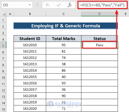
- Firstly, you have to select a different cell D5 where you want to see the Status.
- Secondly, you should use the corresponding formula in the D5
=IF(C5>=60,"Pass","Fail")- Subsequently, you must press ENTER to get the result.
Formula Breakdown
Here, the IF function returns the result which will fulfill a given condition.
- Firstly, the C5>=60 denotes a logical test. Where the function will test that either the Total Marks is greater than or equal to 60.
- Secondly, “Pass” denotes that if the logic is TRUE on C5 then it will give Pass. Here, when you use any string then you must use the Inverted Comma.
- Finally, “Fail” denotes that if the logic is FALSE on C5 then it will give Fail.
- After that, you can double-click on the Fill Handle icon to AutoFill the corresponding data in the rest of the cells D6:D15.
Finally, you will get the Status.

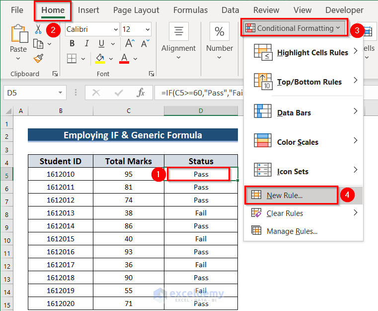
At this time, I will apply Conditional Formatting with formula. Here, I will use a simple equation.
- Firstly, you should select the data at which you want to apply the Conditional Formatting to color the status Pass/Fail. Here, I have selected the data D5 cell.
- Secondly, from the Home tab >> you must go to the Conditional Formatting
- Thirdly, you need to choose the New Rule option to apply the formula.
At this time, a dialog box named New Formatting Rule will appear.
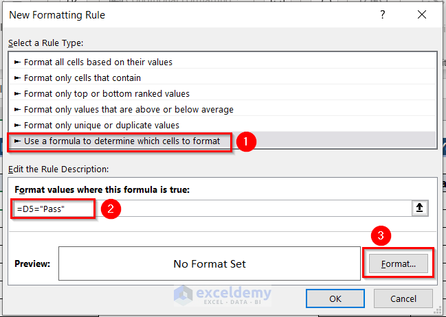
- Now, from that dialog box >> you have to select Use a formula to determine which cells to format.
- Then, you need to write down the following formula in the Format values where this formula is true:
=D5= "Pass"- Here, in the formula, you must use the Inverted Comma.
- After that, go to the Format
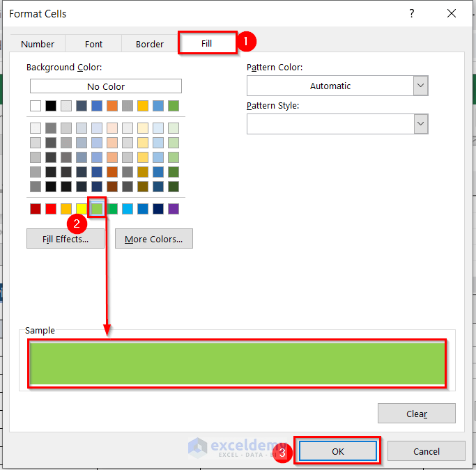
At this time, a dialog box named Format Cells will appear.
- Now, from the Fill option >> you have to choose any of the colors. Here, I have chosen Light Green. Also, you can see the sample In this case, try to choose any light color. Because, the dark color may hide the inputted data. Then, you may need to change the Font Color.
- Then, you must press OK to apply the formation.
- After that, you have to press OK on the New Formatting Rule dialog box. Here, you can see the sample instantly in the Preview

Similarly, go through the previous process to open the window named New Formatting Rule.
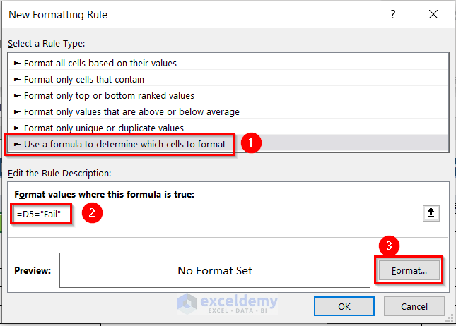
- Now, from that dialog box >> you have to select Use a formula to determine which cells to format.
- Then, you need to write down the following formula in the Format values where this formula is true:
=D5= "Fail"- Here, in the formula, you must use the Inverted Comma.
- After that, go to the Format
At this time, a dialog box named Format Cells will appear.
- Now, from the Fill option >> you have to choose any of the colors. Here, I have chosen Red. Also, you can see the sample
- Then, you must press OK to apply the formation.

- After that, you have to press OK on the New Formatting Rule dialog box. Here, you can see the sample instantly in the Preview
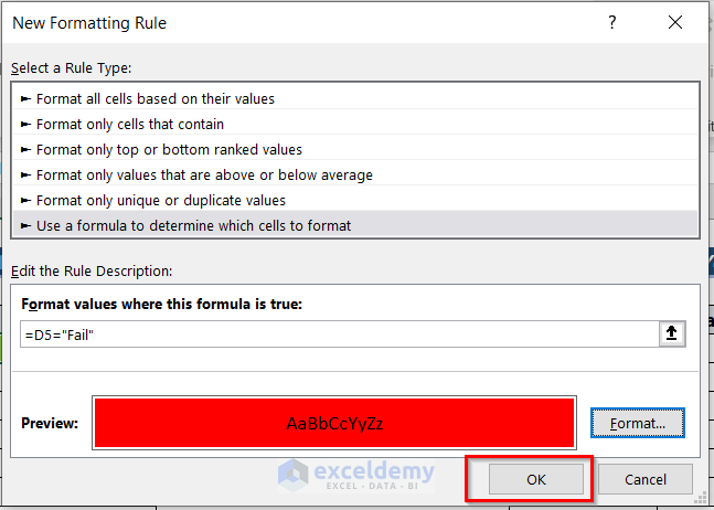
Finally, you will see the colored Pass/Fail.
Read More: Calculate Grade Using IF function in Excel
5. Use of AND, COUNTIF and IF Functions
You can use some combination of functions to fill the Status. Here, I will use AND function, COUNT function, and IF function as Excel Formula for Pass or Fail. Additionally, I have to use Conditional Formatting to color the Status. For this method, let’s have the following dataset. Which contains 4 columns. Those are Student ID, Math, English, and History.

The steps are given below.
Steps:
- Firstly, you have to select a different cell F5 where you want to see the Status.
- Secondly, you should use the corresponding formula in the F5
=IF(AND(COUNTIF(C5:E5,">=60")>=2,C5>=60,D5>=60),"Pass","Fail")- Subsequently, you must press ENTER to get the result.

Formula Breakdown
- Here, COUNTIF(C5:E5,”>=60″) → counts the cells which will fulfill the given condition. The condition says that either the number is greater than or equal to 60.
- Output→ 3
- Again, the AND function will check whether all the conditions are fulfilled or not.
- AND(3)>=2,C5>=60,D5>=60 → checks, firstly is it greater than or equal to 2; secondly is the cell value of C5 greater than or equal to 60; thirdly, is the cell value of D5 greater than or equal to 60.
- Output→ TRUE
- IF function will return Pass when the output is TRUE otherwise return Fail.
- Output→ Pass
- After that, you can double-click on the Fill Handle icon to AutoFill the corresponding data in the rest of the cells F6:F15.
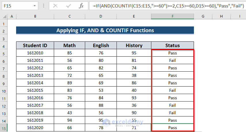
Lastly, you will see the colored Pass/Fail.

Read More: Calculate Letter Grades in Excel
💬 Things to Remember
- According to your dataset, you should choose the method.
Practice Section
Now, you can practice the explained method by yourself.

Download Practice Workbook
You can download the practice workbook from here:
Conclusion
I hope you found this article helpful. Here, I have explained 5 methods to use Excel Formula for Pass or Fail with Color. Please, drop comments, suggestions, or queries if you have any in the comment section below.
Related Articles
- How to Calculate Grades with Weighted Percentages in Excel
- Make a Grade Calculator in Excel
- How to Calculate Percentage of Marks in Excel
- Apply Percentage Formula in Excel for Marksheet
- How to Make Result Sheet in Excel

