How to Apply Percentage Formula in Excel for Marksheet (7 Applications)

In this tutorial, we will show you how to apply the percentage formula in Excel for the marksheet. It’s very easy to create a mark sheet in Microsoft Excel. We will apply multiple formulas to create a simple and dynamic mark sheet. To illustrate the working process of this tutorial we will go over several examples with different types of datasets.


How to Apply Percentage Formula in Excel for Marksheet: 7 Applications

There are different ways to apply the percentage formula in Excel to create a mark sheet. In this article, we will demonstrate 7 different applications of the percentage formula in Excel to create a mark sheet.


1. Fundamental Method of Percentage Formula in Excel for Marksheet

First and foremost, we will apply the basic percentage formula in Excel to create a mark sheet. To calculate what percentage of a number is another number we just have to divide one number with another number and then multiply with 100. If we want to determine what percentage of A is B we will use the following formula.

Fundamental Method of Percentage Formula in Excel for Marksheet

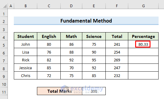
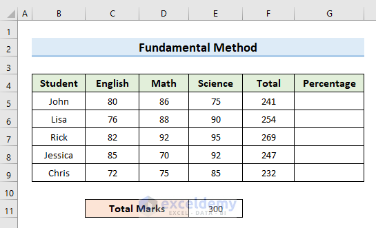
In the following dataset, we have marks for 3 subjects for five students and their total obtained marks. Here, the total mark for 3 subjects is 300. We will calculate what percentage of total marks each student gets.
Fundamental Method of Percentage Formula in Excel for Marksheet

So, let’s take a look at the steps to calculate the percentage of obtained marks for each student.

STEPS:

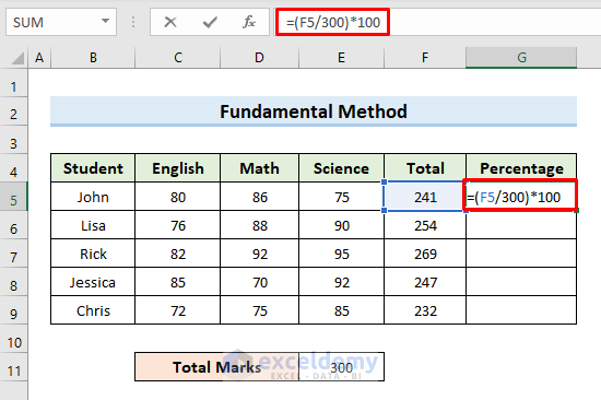
  • Firstly, select cell G5. Insert the following formula in that cell:
=(F5/300)*100
Fundamental Method of Percentage Formula in Excel for Marksheet

  • Now press Enter. This action returns the percentage for the first student.

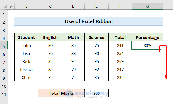
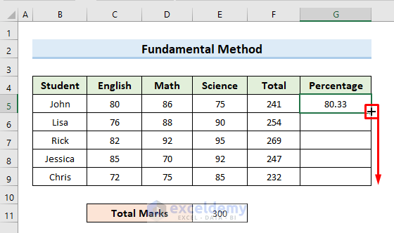
  • Secondly, select cell G5. Move the mouse cursor to the bottom right corner of the selected cell so that it turns into a plus (+) sign like the following image.
  • Thirdly, click on the plus(+) sign and drag the Fill Handle down to cell C9 to copy the formula of cell G5 in other cells. We can also double-click on the plus (+) sign to get the same result.
  • After that, let go of the mouse click.
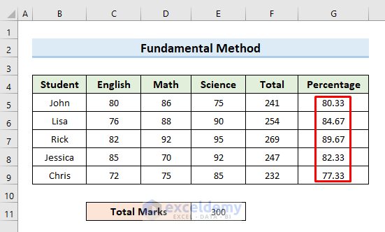
  • Finally, the above command copies the formula of cell G5 to the other cells. So, we can see the percentage of marks for all students.
Fundamental Method of Percentage Formula in Excel for Marksheet

Read More: Make an Excel Spreadsheet Automatically Calculate Percentage


2. Apply Percentage Formula from Excel Ribbon

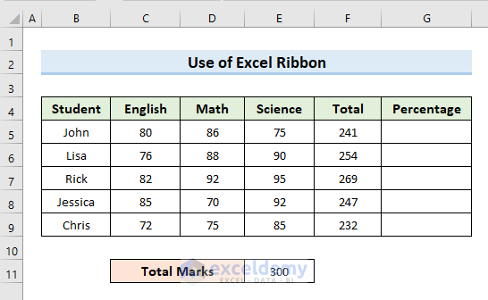
Applying the percentage formula from the Excel ribbon is another fast and convenient way. To demonstrate this, we will calculate the percentage of our previous dataset again. But this time we will do it from the Excel ribbon. The following image is an overview of our previous dataset.
Apply Percentage Formula from Excel Ribbon

Let’s see the steps regarding this method.

STEPS:

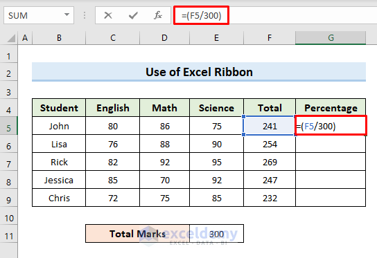
  • First, select cell G5. Insert the following formula in that cell:
=(F5/300)
  • If you notice you will see we have not multiplied the value by 100 here like the previous example.
Apply Percentage Formula from Excel Ribbon

  • Next, press Enter. This returns the value in decimals.
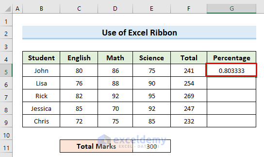
Apply Percentage Formula from Excel Ribbon

  • Then go to the Home tab.
  • Select the option Percent Style(%) or we can do the same action by pressing Ctrl + Shift + % after selecting the cell G5.
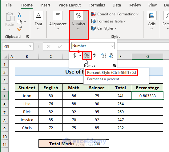
  • So, the above action converts the decimal value into a percentage.
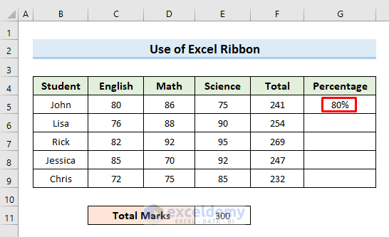
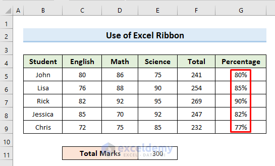
  • After that, select cell Drag the Fill Handle tool to cell G9 and release the mouse click.

  • Finally, the above command returns all the values in percentage.

Apply Percentage Formula from Excel Ribbon

Related Content: How to Apply Percentage Formula for Multiple Cells in Excel


3. Extract Particular Value Using Percentage Formula in Excel

In the previous two examples, we have used the percentage formula to calculate the percentage. Now, in this example, we will use the percentage value to extract amounts and totals.

3.1 Evaluate Individual Marks by Total and Percentage

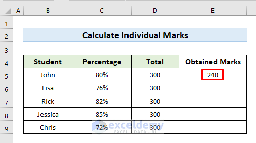
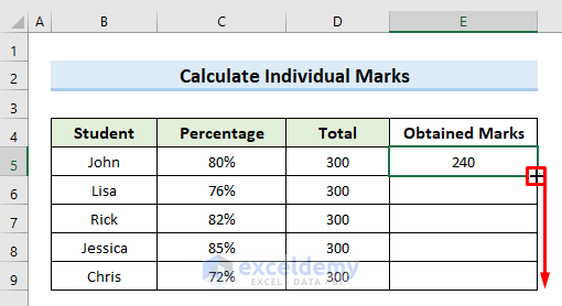
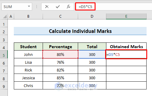
In the following dataset, we have the total marks and percentages gained by all students. From these two values, we will calculate the Obtained Marks for each student.
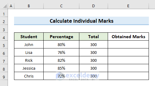
Evaluate Individual Marks by Total and Percentage

So, let’s see the steps to do this method.

STEPS:

  • In the beginning, select cell E5. Insert the following formula in that cell:
=D5*C5
Evaluate Individual Marks by Total and Percentage

  • Now, hit Enter. This action returns the obtained mark for the first student.

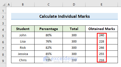
  • After that, select cell Drag the Fill Handle tool to cell E9 and release the mouse click.

  • Finally, The above action return obtained marks for all students in cells (G5:G9).
Evaluate Individual Marks by Total and Percentage


3.2 Use Individual Marks and Percentage to Evaluate Total Marks

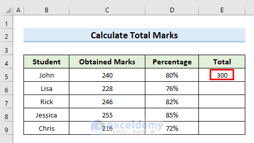
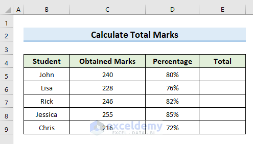
For this method, we have the value of Obtained Marks & Percentage in our following dataset. We will calculate the total marks by using these two values.
Use Individual Marks and Percentage to Evaluate Total Marks

Let’s look at the steps to perform this action.

STEPS:

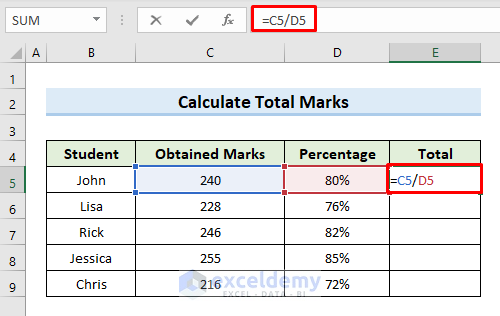
  • Firstly, select cell E5. Insert the following formula in that cell:
=C5/D5
Use Individual Marks and Percentage to Evaluate Total Marks

  • Now, press Enter. This action returns the value of the total mark.

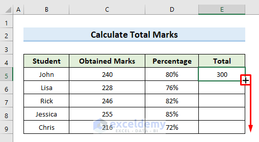
  • Secondly, select cell Drag the Fill Handle tool to cell E9 and release the mouse click.

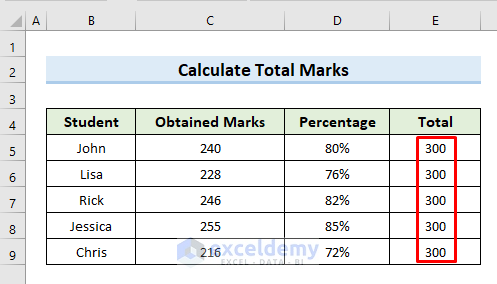
  • Lastly, the above command returns the value of total marks in cell (E5:E9).

Use Individual Marks and Percentage to Evaluate Total Marks

Read More: How to Calculate Total Percentage in Excel


4. Use Percentage Formula in Excel to Modify Existing Marks by a Percentage

Sometimes we need to modify the values of the mark sheet by a fixed percentage. So, in this section, we will explain how to modify an existing value of a mark sheet by a specific percentage.

4.1 Increase Marks by a Percentage

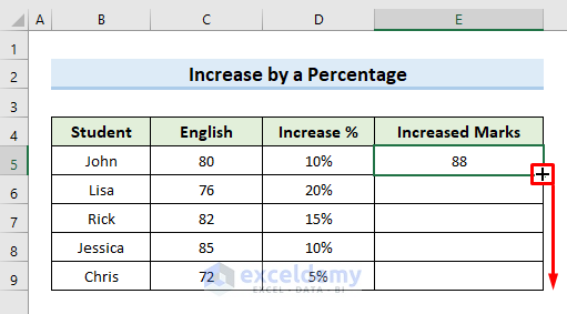
We have the following dataset, which contains the obtained marks for six students in the subject of English. Here, we will increase the marks of each student by different percentages.
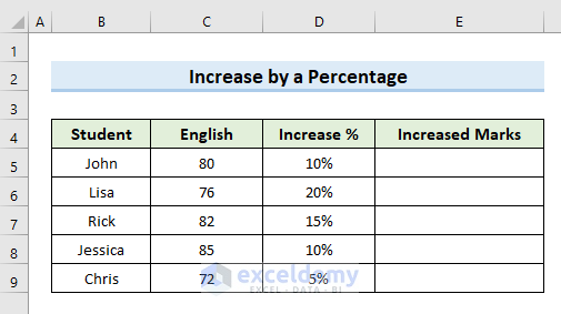
Increase Marks by a Percentage

So, let’s see the steps to how to perform this method.

STEPS:

  • First, select cell E5. Insert the following formula in that cell:
=C5*(1+D5)
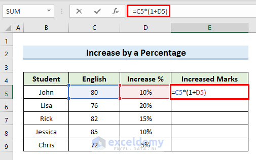
Increase Marks by a Percentage

  • Now, hit Enter. We get the increased value in cell E5.
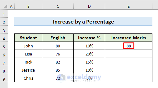
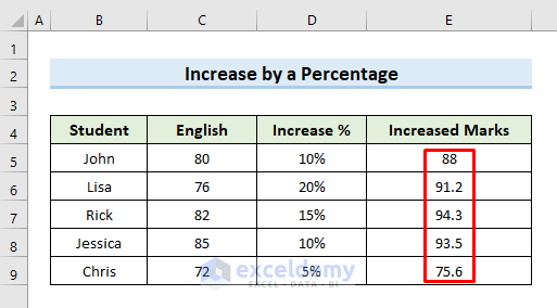
  • After that, select cell Drag the Fill Handle tool to cell E9 and release the mouse click.

  • Lastly, we can see the increased value of marks by corresponding percentages in cells (E5:E9).

Increase Marks by a Percentage


4.2 Decrease Marks by a Percentage

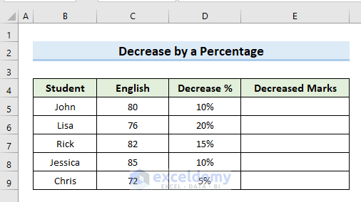
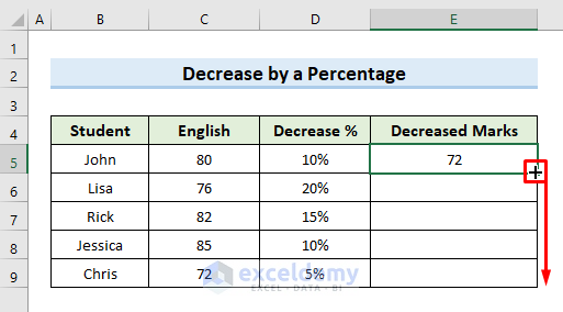
If we look at the following dataset this method is just the reverse of our previous method. In this method, we will decrease the value of obtained marks by a specific percentage whereas in the previous method, we calculated increased marks.

Decrease Marks by a Percentage

So, let’s look at the steps to execute this method.

STEPS:

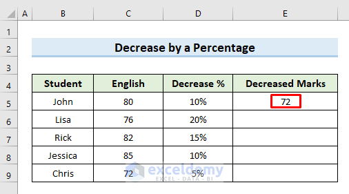
  • In the beginning, select cell E5. Insert the following formula in that cell:
=C5*(1-D5)
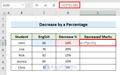
Decrease Marks by a Percentage

  • Now, press This action to return the marks in cell E5.

  • Next, select cell Drag the Fill Handle tool to cell E9 and free the mouse click.

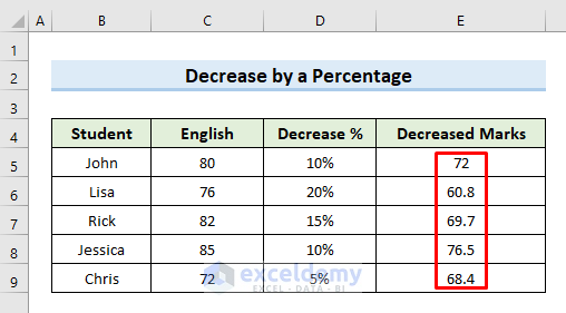
  • Finally, we can see the decreased marks for all students in cell (E5:E9).

Decrease Marks by a Percentage


5. Modify the Entire Column of a Marksheet by Using Percentage Formula in Excel

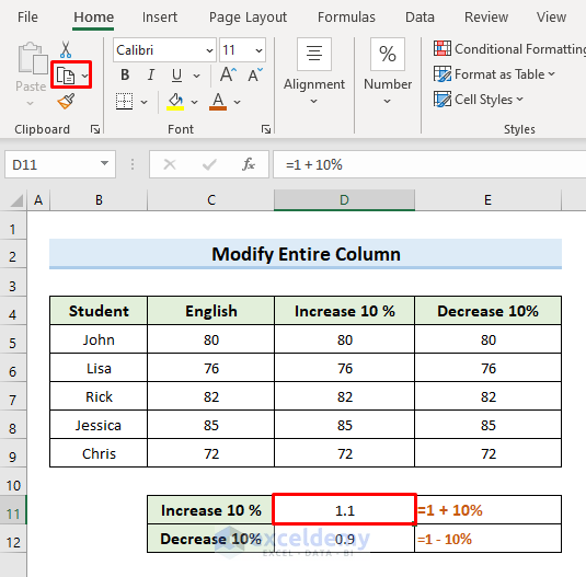
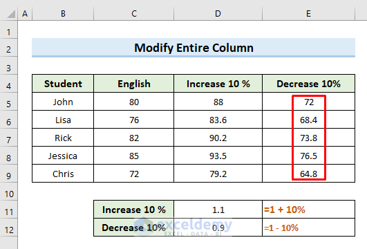
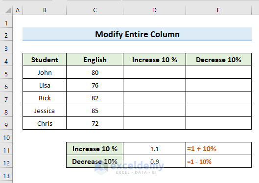
In this example, we will modify an entire column by a single percentage. In the following dataset, we have a mark sheet of six students containing their marks in English. So, to clarify this method we will increase and decrease the marks of all students by 10%.
Modify the Entire Column of a Marksheet by Using Percentage Formula in Excel

Let’s take a look at the steps regarding this method.

STEPS:

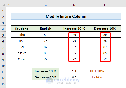
  • Firstly, copy the same value of marks in the columns “Increased 10%” and “Decreased 10%”.
Modify the Entire Column of a Marksheet by Using Percentage Formula in Excel

  • Secondly, increasing 10% means taking multiplies as 2, and Decreasing 10% means taking the multiplier as 0.9.
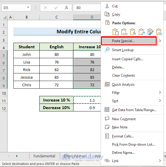
  • Thirdly, select cell D11. Click on the Copy from ribbon or you can press Ctrl + C.

Modify the Entire Column of a Marksheet by Using Percentage Formula in Excel

  • Now, a new dialogue box will appear. Check the option “Multiply” from that box.
  • Then press OK.

  • So, the above command increases all the values of cells (D5:D9) by 10%.
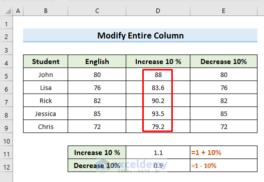
  • Lastly, take the value of multiplier 9 and follow the same process to modify the value of the cell (E5:E9).

Modify the Entire Column of a Marksheet by Using Percentage Formula in Excel


6. Create Dynamic Marksheet in Excel

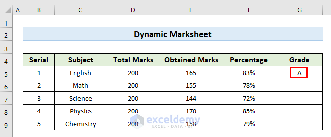
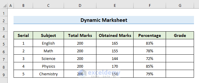
In this example, we will create a dynamic mark sheet by using the percentage formula. Using the dynamic mark sheet, we will get grades automatically with the change of percentages. In the following dataset, we will input the values of grades according to their percentages.
Create Dynamic Marksheet in Excel

Let’s see the steps of how we can create a dynamic mark sheet.

STEPS:

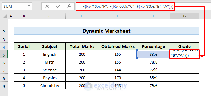
  • First, select cell G5 and insert the following formula:
=IF(F5<40%,"F",IF(F5<60%,"C",IF(F5<80%,"B","A")))
Create Dynamic Marksheet in Excel

  • Now, hit Enter. This action reciprocates the grade value A since the percentage is above 80%.

Create Dynamic Marksheet in Excel

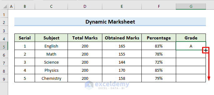
  • Next, select cell Drag the Fill Handle tool to cell G9 and release the mouse click.

  • So, we can see the grades for all students in the column “Grade”.
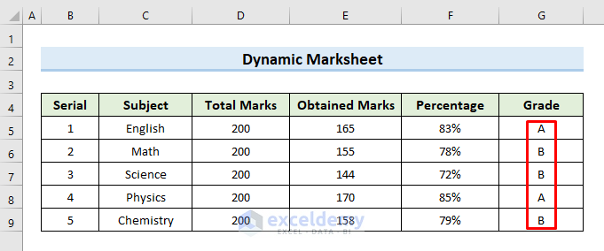
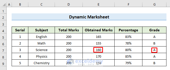
  • Lastly, if we change the marks in cell E7 from 144 to 160, the grades will automatically change from B to A.
Create Dynamic Marksheet in Excel

The conditions that we have used in the formula:

If the percentage is > 80% it will return A, if the percentage is < 80% it will return B, if the percentage is < 60% it will return C, if the percentage is < 40% it will return F.

Read More: How to Calculate Grade Percentage in Excel


7. Error Handling While Using Percentage Formula in Excel

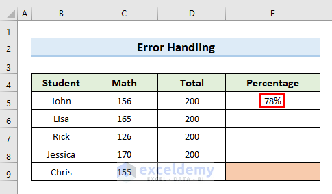
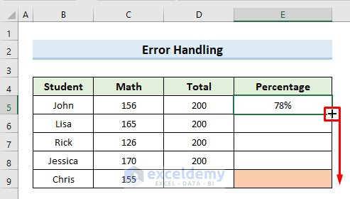
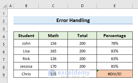
While applying the percentage formula to create a mark sheet in Excel we may face errors sometimes. In this article, we will explain how we can handle these errors by using the IFERROR function. The IFERROR function returns another value if the formula returns an error value. In the following dataset, we face an error in the last row because cell value D9 is missing.
Error Handling While Using Percentage Formula in Excel

So, let’s see the steps of how we can handle errors in the percentage formula.

STEPS:

  • Firstly, select a cell Insert the following formula in that cell:
=IFERROR(C5/D5,0)
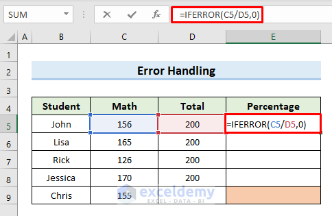
Error Handling While Using Percentage Formula in Excel

  • Now, press Enter. This returns the percentage value for the marks of the first student.

  • Next, select cell Drag the Fill Handle tool to cell E9 and free the mouse click.

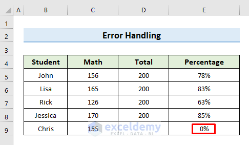
  • Finally, we can see the value 0 in place of the “#DIV/0” Here the IFERROR formula returns 0 since the original formula returns an error.

Error Handling While Using Percentage Formula in Excel


Download Practice Workbook

You can download the practice workbook from here.


Conclusion

At last, this post will show you how to apply the percentage formula in Excel for mark sheets. Download the practice workbook that comes with this article to test your skills to the test. If you have any questions, please leave a comment in the box below. We’ll do our best to respond as soon as possible. Keep an eye out for more intriguing Microsoft Excel solutions in the future.


Related Articles


<< Go Back to Percentage Formula ExamplesCalculating Percentages | Calculate in Excel | Learn Excel

Get FREE Advanced Excel Exercises with Solutions!
Mukesh Dipto
Mukesh Dipto

Mukesh Dipto is an excellent marine engineer who loves working with Excel and diving into VBA programming. For him, programming is like a superhero tool that saves time when dealing with data, files, and the internet. His skills go beyond the basics, including Rhino3D, Maxsurf C++, AutoCAD, HTML, CSS, JavaScript, and WordPress. He got his B.Sc in Naval Architecture & Marine Engineering from BUET, and now he's switched gears, working as a content developer. In this role, he... Read Full Bio

We will be happy to hear your thoughts

Leave a reply

Advanced Excel Exercises with Solutions PDF


ExcelDemy
Logo