How to Apply a Percentage Formula in Multiple Cells in Excel – 5 Methods

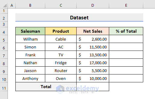
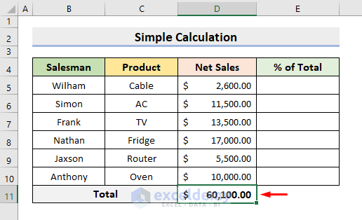
The sample dataset showcases Salesman, Product, and Net Sales of a company.

Method 1 – Using the Excel Division Symbol and the Percentage Format to Apply the Percentage Formula in Multiple Cells

STEPS:

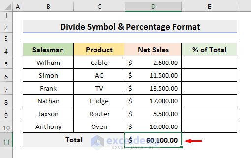
• Select D11. Enter the formula:

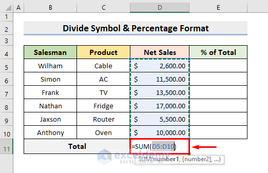
• Press Enter.

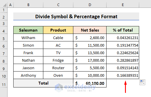
• Select E5. Enter the formula:

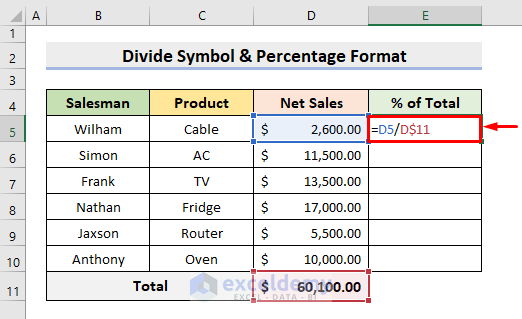
• Press Enter.
• Drag down the Fill Handle to see the result in the rest of the cells.

• Select the range of cells to convert to percentage format.

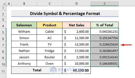
• Select the ‘%’ icon in Number.

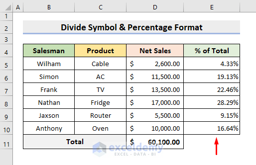
This is the output.

Read More: Make an Excel Spreadsheet Automatically Calculate Percentage

Method 2 – Applying a Percentage Formula Manually in Multiple Cells

STEPS:

• Select D11. Enter the formula:

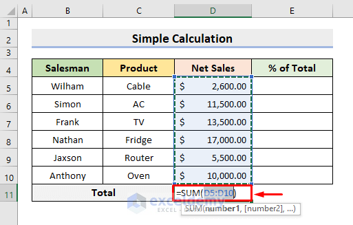
• Press Enter to see the Sum of Net Sales.

• Select E5. Enter the formula:

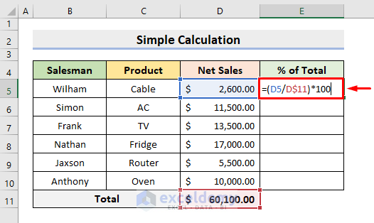
• Press Enter.
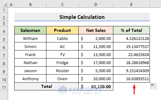
• Drag down the Fill Handle to see the result in the rest of the cells.

This is the output.

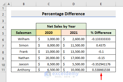
Method 3 – Using an Excel Percentage Formula in Multiple Cells by Calculating the Percentage Differences

• Select E5. Enter the formula:

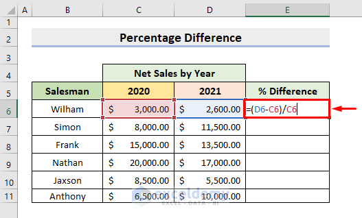
• Press Enter.
• Drag down the Fill Handle to see the result in the rest of the cells.

• Select the range of cells to convert to percentage.

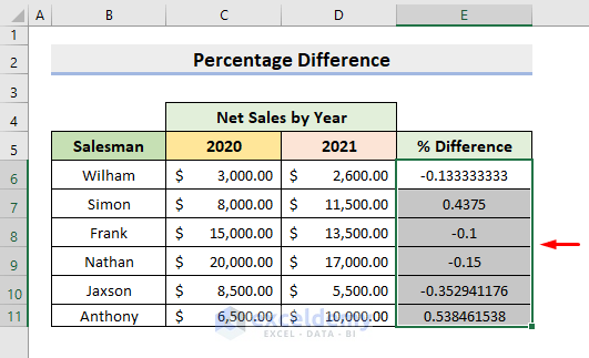
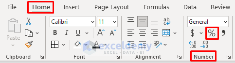
• Select the ‘%’ icon in Number.

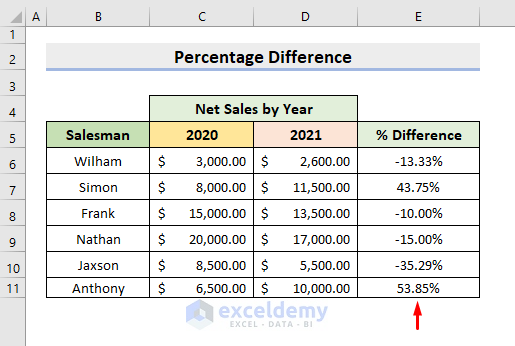
This is the output.

Read More: How to Calculate Percentage for Multiple Rows in Excel

Method 4 Using the Excel SUMIF Function to Apply a Percentage Formula in Multiple Cells

You want to find Wilham’s impact in the percentage of the total sales.

STEPS:

• Select D11. Enter the formula:

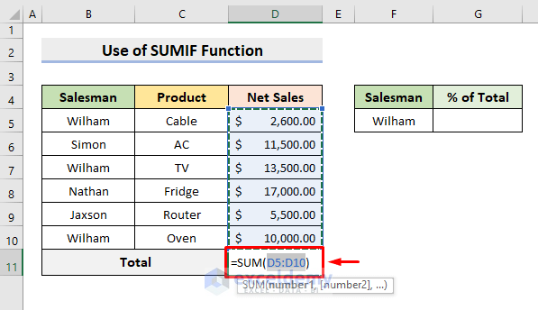
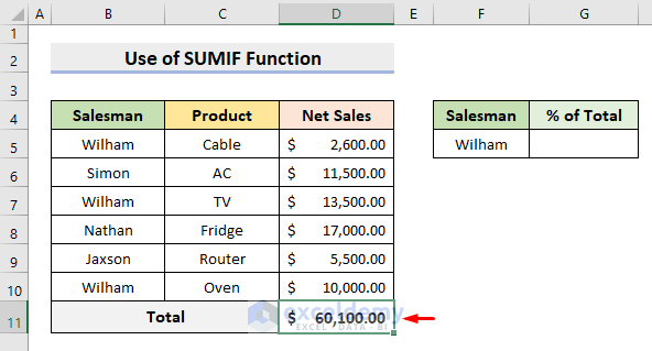
• Press Enter to see the sum.

• Select G5. Enter the formula:

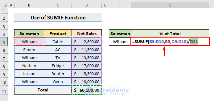
• Press Enter.
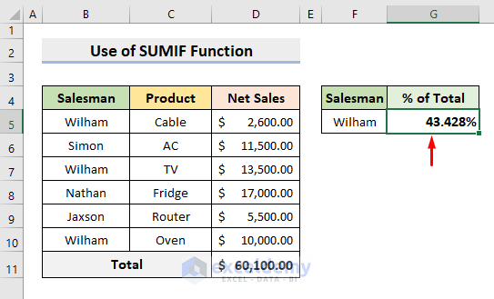
• Select the ‘%’ icon in Number.

• Wilham’s contribution to the total sales is displayed.

Method 5- Using an Increasing/Decreasing Percentage Formula

STEPS:

• Select F5. Enter the formula:

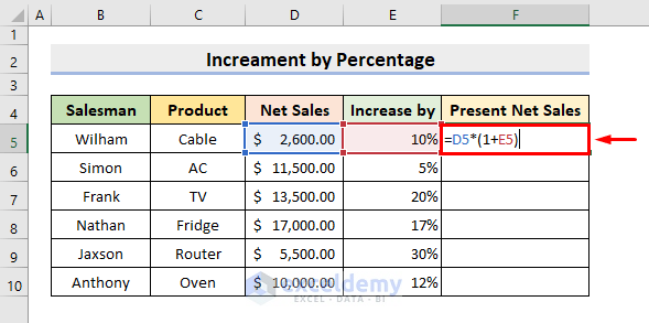
• Press Enter. Drag down the Fill Handle to see the result in the rest of the cells.
• This is the output.

Download Practice Workbook

Practice with the following workbook.

Related Articles

• Calculate Percentage Using Absolute Cell Reference in Excel
• Calculate Percentage in Excel VBA
  
• How to Calculate Percentage of Filled Cells in Excel
• IF Percentage Formula in Excel
• How to Find the Percentage of Two Numbers in Excel
• How to Calculate Contribution Percentage with Formula in Excel
• How to Use Food Cost Percentage Formula in Excel
• How to Calculate Percentage above Average in Excel
• How to Apply Percentage Formula in Excel for Marksheet
• How to Calculate Variance Percentage in Excel

<<Go Back to Calculating Percentages in Excel | How to Calculate in Excel | Learn Excel