How to Find the Percentage of Two Numbers in Excel

Method 1 – Using a Formula to Find a Percentage of Two Numbers

Steps:

• Choose a cell (E5) and apply the following formula-

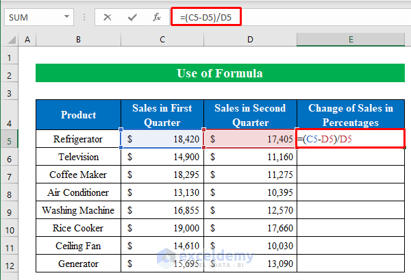
• Hit ENTER and drag the “Fill Handle” down to fill all the cells.

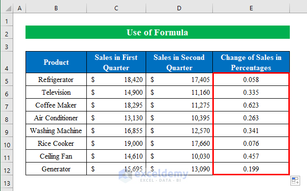
• Change the output to percent style by choosing cells (E5:E12) and clicking the “Percent Style” icon from the Home tab.

• Here’s the result.

Method 2 – Applying a Keyboard Shortcut to Find the Percentage of Two Numbers

Steps:

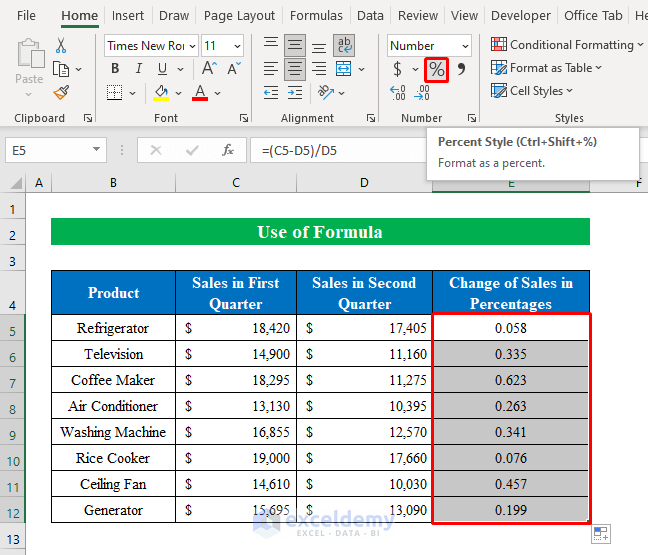
• Choose a cell (E5) and apply the following formula.

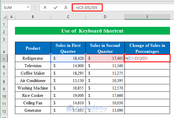
• Click ENTER and pull the “Fill Handle” down.
• While the output cells (E5:E12) are selected, press CTRL + SHIFT + % from the keyboard.

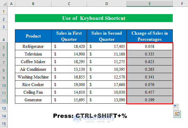
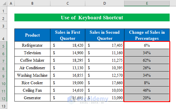
• Our result is ready with a simple shortcut.

Method 3 – Finding Percentage of Two Numbers in Different Excel Rows

Steps:

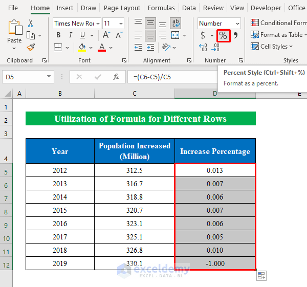
• Select a cell (D5) and insert the following:

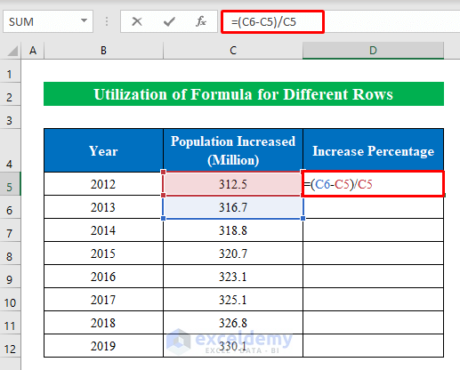
• Hit ENTER and drag down the “Fill Handle” to fill all the cells with the proper output.

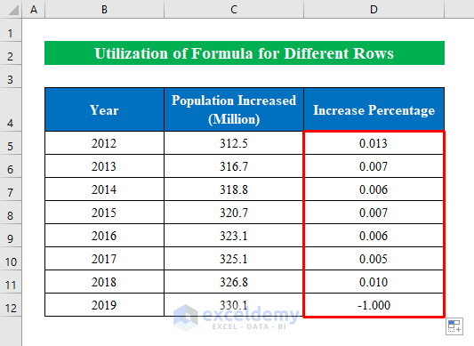
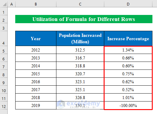
• Selecting cells (D5:D12) change the style to “Percent Style” by hitting the “Percent” icon from the top ribbon.

• We have found the percentage of two numbers for different rows.

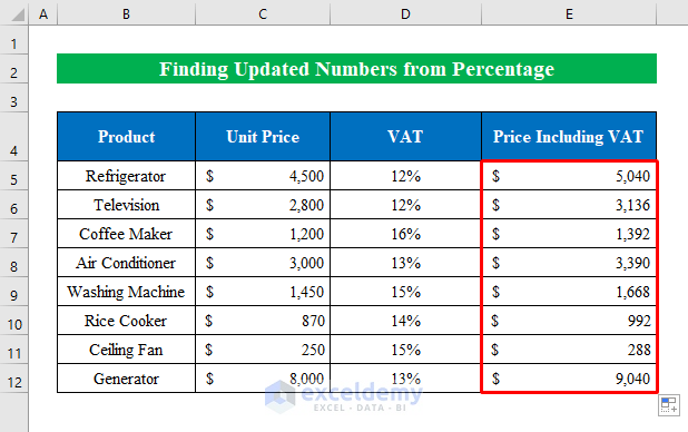
Finding Updated (Increment or Decrement) Numbers with a Percentage in Excel

Steps:

• Choose a cell (E5) and apply the following formula.

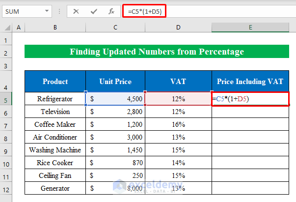
• Hit ENTER and drag down the “Fill Handle”.
• We got our increment output from the percentage value.

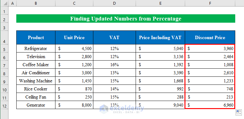
• To find the updated decreased value with percentage, choose a cell (F5) and use the following:

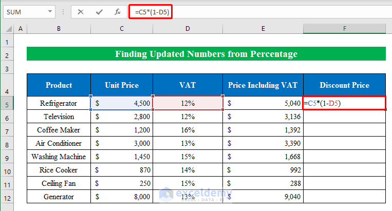
• Click ENTER and fill down the cells by dragging the “Fill Handle”.
• We have our decreased output in our hands.

Use the Format Cells Feature to Mark Percentages of Two Numbers

Steps:

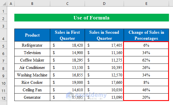
• Choose a cell (E5) and apply the following formula-

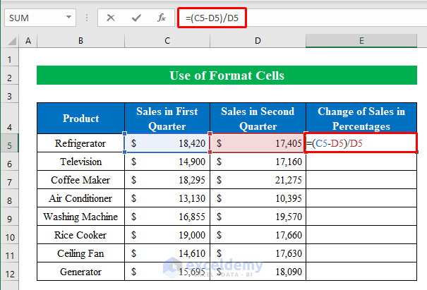
• Press ENTER and drag the “Fill Handle” down.
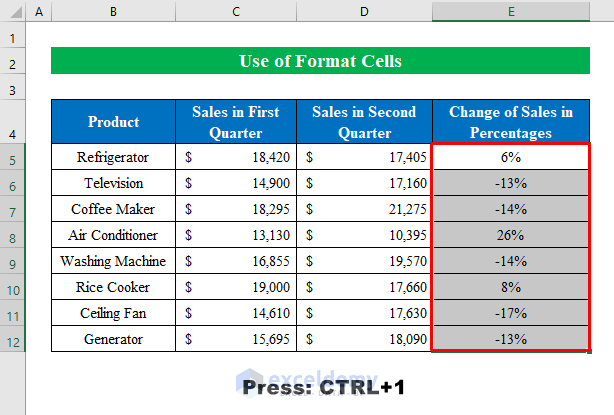
• While the output is selected, click the “Percent Style” icon from the top ribbon.

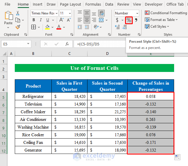
• We have got our output in percentages.
• After choosing all output results, press CTRL+1 to go to the “Format Cells” window.

• In the new window, choose “Custom” and type “00%;[Red]-0.00%”.
• Press OK.

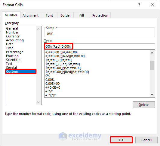
• This marked all the negative percentage values in red.

Download the Practice Workbook

Related Articles

• How to Calculate Total Percentage from Multiple Percentages in Excel
• How to Calculate Percentage of Month in Excel
• How to Calculate Percentage of Percentage in Excel
• How to Calculate Percentage Based on Conditional Formatting
• How to Calculate Percentage in Excel Based on Cell Color
• Percentage Showing as Thousand in Excel
• Why Are My Percentages Wrong in Excel?
• How to Remove Percentage in Excel
• How to Calculate Percentage Complete Based on Dates in Excel
• How to Calculate Error Percentage in Excel
• How to Calculate Cumulative Percentage in Excel

<<Go Back to Calculating Percentages in Excel | How to Calculate in Excel | Learn Excel