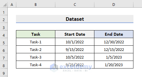
A starting and an ending date are needed. We’ll use the TODAY function for the current date. You can input any date. To illustrate, we’ll use the following dataset as an example..
Note that,
- If the TODAY function returns a date value between the start and end dates, you will get the intended percentage value.
- When TODAY is greater than the end date, we will get 100% or more than 100%, meaning the task is complete.
- If TODAY is less than both the start and end dates, we will get negative values or negative percentage values (which means the tasks have not started yet).
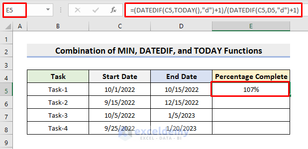
Method 1 – Combining the DATEDIF and TODAY Functions to Calculate Percentage Completed Based on Dates
The DATEDIF function can determine the number of days, months, and years between the two dates to be inserted in the function argument. Method 1 combines the DATEDIF and TODAY functions to create a formula. .
STEPS:
- Select cell E5.
- Type the formula:
=(DATEDIF(C5,TODAY(),"d")+1)/(DATEDIF(C5,D5,"d")+1)
- Press Enter.
- Use AutoFill to populate the rest of the column.
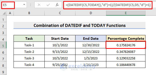
- NOTE: DATEDIF(C5,TODAY(),”d”)+1 part of the formula finds out the number of days between the start date and today. Here, we add 1 to include today’s date. Next, DATEDIF(C5,D5,”d”)+1 determines the total duration of the project. Afterward, we divide the formula outputs to get the ratio of completion.
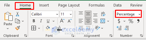
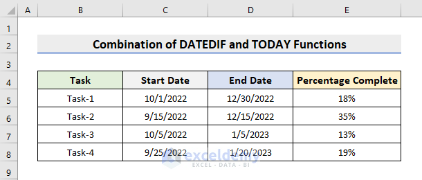
- Go to Home > Number and choose Percentage.
Method 2 – Determine Percentage Complete Based on Dates by Nesting the MIN, DATEDIF, and TODAY Functions
If today is past the end date, the previous formula will give a bizarre result as seen below. To avoid such unwanted errors use the MIN function. This function compares the numbers in its argument and returns the minimum.
To combine the MIN, DATEDIF, and TODAY functions to compute the precise percentage completed follow the steps below.
STEPS:
- Click on cell E5.
- Insert the formula:
=MIN((DATEDIF(C5,TODAY(),"d")+1)/(DATEDIF(C5,D5,"d")+1),100%)
- Hit Enter and use AutoFill.

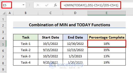
Method 3 – Create Formula Using Excel MIN and TODAY Functions for Calculating Percentage Complete
Moreover, the MIN and TODAY functions can also do the same job of determining the percentage complete. The formula is smaller too. Hence, follow the process below.
STEPS:
- Select cell E5.
- Input the formula:
=(MIN(TODAY(),D5)-C5+1)/(D5-C5+1)
- Press Enter.
- Apply AutoFill to complete the rest.
Read More: How to Calculate Contribution Percentage with Formula in Excel
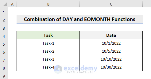
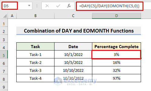
Method 4 – Get Percentage Completed Using the DAY and EOMONTH Functions
We’ll assume that the duration of each of the tasks below is a month. The given Date is the reference up to which the work is completed. The DAY function extracts the day from a date and the EOMONTH function finds out the last date of a specified month. To calculate the percentage complete, we’ll join these two functions. .
STEPS:
- Choose cell D5.
- Input the formula:
=DAY(C5)/DAY(EOMONTH(C5,0))
- Press Enter.
- Apply AutoFill to fill the series.
- Where we demonstrate the results.
Download Practice Workbook
Download the following workbook to practice by yourself.
Related Articles
- How to Calculate Total Percentage from Multiple Percentages in Excel
- How to Calculate Percentage of Month in Excel
- How to Calculate Percentage of Percentage in Excel
- How to Calculate Percentage Based on Conditional Formatting
- How to Calculate Percentage in Excel Based on Cell Color
- Percentage Showing as Thousand in Excel
- Why Are My Percentages Wrong in Excel?
- How to Remove Percentage in Excel
- How to Find the Percentage of Two Numbers in Excel
- How to Calculate Error Percentage in Excel
- How to Calculate Cumulative Percentage in Excel
<<Go Back to Calculate Percentage with Criteria in Excel | Calculating Percentages in Excel | How to Calculate in Excel | Learn Excel
Get FREE Advanced Excel Exercises with Solutions!

Hello, I have a spreadsheet where I log completed training of a large number of people and teams. Each team has it’s own spreadsheet. There are a number of courses each person has to complete. I have set the spreadsheet up to make the cell go red if the person is out of date on a course and needs to repeat it and green if they are in date. How can I show the percentage completed for each course both for each team and again for the organisation as a whole?
Hello SAZ,
Greetings. Using Excel formulas and charts, you can display the percentage of each course that has been completed for each team and the entire organization. The steps are as follows:
1) Calculate the percentage completed for each course for each person:
You can use a formula to count the number of completed courses and divide it by the total number of courses for each person. For example, if the number of courses is in column B and the completed courses are in column C, the formula in column D could be:
=IFERROR(C2/B2,0)
Calculate the percentage completed for each course for each team:
2) You can use the AVERAGEIF function to calculate the average percentage completed for each course for each team. For example, if the team name is in column A and the percentage completed is in column D, the formula in column E could be:
=IFERROR(AVERAGEIF(A:A,A2,D:D),0)
Calculate the percentage completed for each course for the organization as a whole:
You can use the same AVERAGEIF function to calculate the average percentage completed for each course for the entire organization. For example, if the percentage completed is in column D, the formula in column E could be:
=IFERROR(AVERAGEIF(D:D,”>0″),0)
Create a chart:
3) You can create a column chart to visualize the percentage completed for each course for each team and for the organization as a whole. Select the data range that includes the course names and the percentage completed columns, then go to Insert > Charts > Column Chart and choose the type of chart you prefer. You can also add labels, titles, and legends to the chart as needed.
With the help of these steps, you ought to be able to monitor the percentage of each course that has been completed by each team and the organization as a whole.
Hello, I’m trying to insert the formulas in excell, but it doesn’t work, I get this error message: “There is a problem with this formula.” I’ve tried to insert the dates as dates and texts, but the same error appears. Any idea how I can solve it?
Hello TANJA,
Hope you are doing good. Thanks for your query.
specifically, which method’s formula isn’t working for you? If you said that, I could understand well. Because all formulas are working on my PC.
The error message “There is a problem with this formula” usually appears when there is an issue with the syntax of the formula. If we take Method 2 as example, the following is the formula we used in cell E5:
=MIN((DATEDIF(C5,TODAY(),"d")+1)/(DATEDIF(C5,D5,"d")+1),100%)It’s possible that the issue is related to the regional settings or the version of Excel being used on your PC. The formula we are using includes a percentage sign (“%“), which represents a percentage value. Depending on the regional settings or version of Excel being used, the formula may not recognize the percentage sign as a valid argument. To avoid any potential compatibility issues, you can modify the formula to use a decimal value instead of a percentage. For example, you can use “1” to represent 100%. I just told it as an example. It could be better if you tell me which formula isn’t working and which Excel version are you using.
Hope you can understand me. Happy Excelling.
Regards,
SHAHRIAR ABRAR RAFID
Team ExcelDemy
Hi – I have this formula for % completed between two dates in a project plan. I also added a iferror statement that if the dates are TBD it would return a 0%. Now I need to cap the percentages to 100%. Can you help with the right formula?
=IFERROR((DATEDIF(W6,TODAY(),”d”)+1)/(DATEDIF(W6,X6,”d”)+1),0%)
Hlw Terrisa,
Thank you very much for your comment. The right formula for your need is given below-
=IFERROR(MIN((DATEDIF(W6,TODAY(),”d”)+1)/(DATEDIF(W6,X6,”d”)+1), 1), 0)
Here, we add the MIN function to cap the calculated percentage to 100%. If the calculated percentage is greater than 100%, this function will return 100%, capping the percentage. If the calculated percentage is less than or equal to 100%, it will return the calculated percentage as it is.
If you have other queries let me know in the comment.
Regards,
Sajid Ahmed
Exceldemy
Hello there!
I tried the formula Min-Today, but it’s giving the result 100%, always.
The formula has no error but the formula make is wrong. please note it.
Hello Nadeem Khatri
Thanks for reaching out and posting your comment. You are right about the Percentage Completion column showing 100%. Thank you once again for noticing the interesting issue. You are also correct about the formula used in the article having no error.
Reason: The Percentage Completion column shows 100% for each task. It is important to note that we are using TODAY as a reference day. All the tasks are completed 100% for the dataset shown in the article according to today’s dates.
Note:
Things to Remember:
When inserting date values within the start date and end date columns, ensure all the dates are in the same format.
Solution:
To demonstrate, I am using the dataset mentioned in this article. However, I will use some other date values. Here, you will see an improved version of the formula mentioned in the article to avoid negative values.
Select cell E5 >> apply the following formula >> drag Fill Handle to cell E8.
I hope the idea and concept are crystal clear to you now. Stay Blessed.
Regards
Lutfor Rahman Shimanto