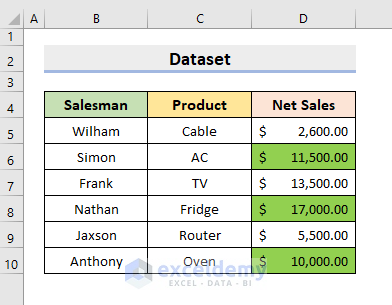
To illustrate our methods for calculating percentage based on cell color, we’ll use the following sample dataset representing the Salesman, Product, and Net Sales of a company. We have colored the net sales of some salesman. Let’s calculate the percentage of the total net sales that the colored net sales comprise.
What is Percentage?
A number or ratio expressed as a fraction of 100 is known as a Percentage. The sign for percentage is ‘%’. The basic percentage is calculated by the formula:
Percentage = (Part / Whole)*100
Calculating Percentage Based on Cell Color
Method 1 – Using the SUBTOTAL Function
We’ll use the Excel SUBTOTAL function along with the Filter feature here.
STEPS:
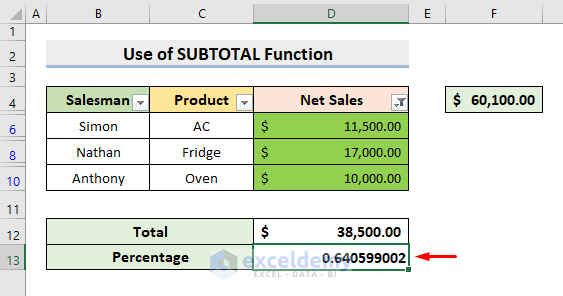
- Select cell D12 and enter the formula:
=SUBTOTAL(9,D5:D10)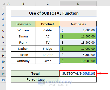
Here, 9 is the function number for SUM and D5:D10 is the range of cells.
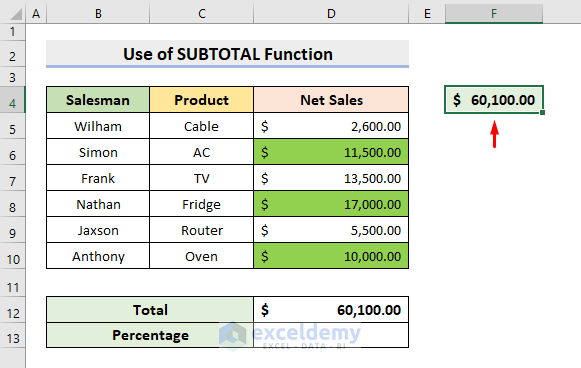
- Press Enter to return the sum result.
- Copy the result and paste it as a value in cell F4.
- Select the range of cells you want to work with.
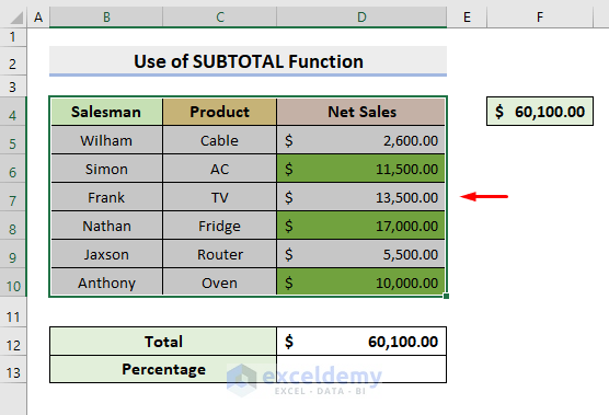
- Select Filter from the Sort & Filter drop-down in the Editing group under the Home tab.
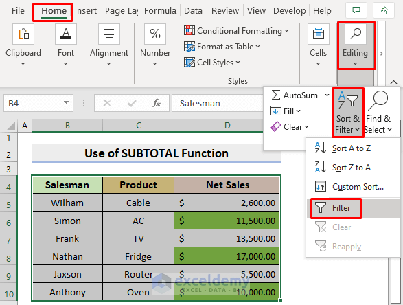
- Select the drop-down icon beside Net Sales.
- Select the Green colored box in the Filter by Cell Color options.
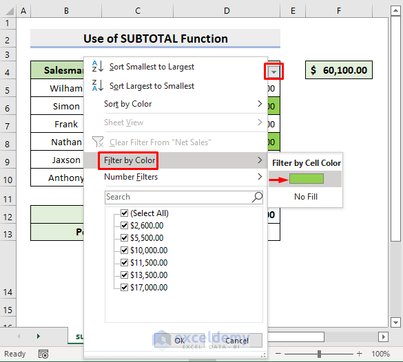
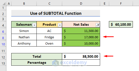
You’ll see the Green colored cells only.
Additionally, the sum result in cell D12 will get updated automatically, and now it’ll return the sum of those green-colored cells only.
- Select cell D13 and enter the formula:
=D12/F4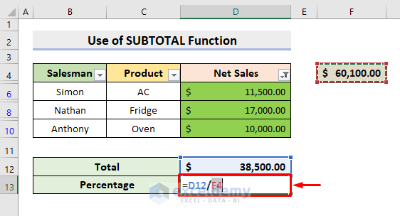
- Press Enter.
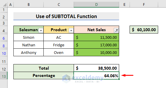
- Select the ‘%’ icon in the Number group under the Home tab.

The desired percentage value of green-colored cells will be returned.
Related Content: How to Calculate Percentage Complete Based on Dates in Excel
Method 2 – Using the SUMIF Function
The SUMIF function computes the sum of a range of cells based on a specific condition given in the argument.
STEPS:
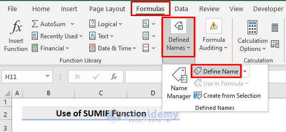
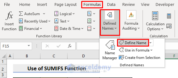
- Select Define Name from the Define Names drop-down under the Formulas tab.
A dialog box will pop out.
- There, enter ColoredNumber in the Name section.
- In the Refers to section, enter the formula:
=GET.CELL(38,‘sumif’!$D5)- Click OK.
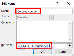
Here, the GET.CELL function takes 38 to return the code color, sumif is the name of the worksheet and D5 is the cell reference.
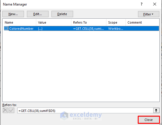
A Name Manager dialog box will pop out
- Click Close.
- Select cell E5 and enter:
=ColoredNumber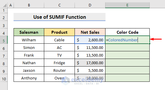
- Press Enter and use the AutoFill tool to fill the series.
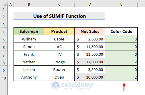
The color codes will be returned.
- Select cell D12 and enter the formula:
=SUM(D5:D10)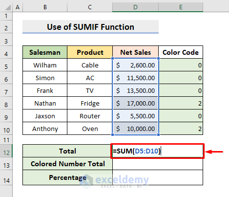
- Press Enter.
- Select cell D13 and enter the formula:
=SUMIF(E5:E10,E8,D5:D10)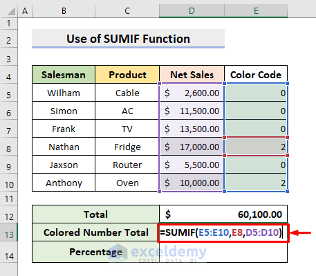
Here, E5:E10 is the criteria range, E8 is our criteria and D5:D10 is the sum range.
- Press Enter.
- Select cell D14 and type the formula:
=D13/D12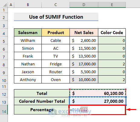
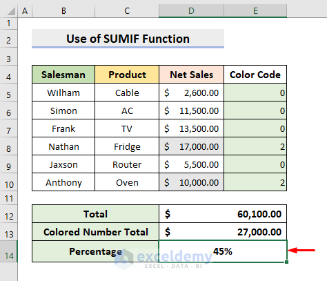
- Press Enter and select the ‘%’ icon in the Number group under the Home tab.

The accurate percentage result will appear in cell D14.
Related Content: How to Calculate Percentage Based on Conditional Formatting
Method 3 – Using the Excel SUMIFS Function
STEPS:
- Select Define Name from the Define Names drop-down under the Formulas tab.
A dialog box will pop out.
- In the Name section, enter ColorCode.
- In the Refers to section, enter the formula:
=GET.CELL(38,sumifs!$D5)- Press OK.
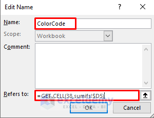
Here, the GET.CELL function takes 38 to return the code color, the name of the worksheet is sumifs and Cell D5 is the cell reference.
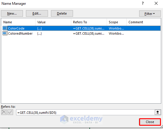
A Name Manager dialog box will pop out.
- Click Close.
- Select cell E5 and enter:
=ColorCode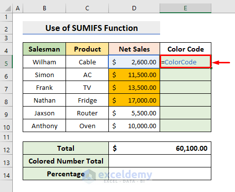
- Press Enter and use the AutoFill tool to fill the series.
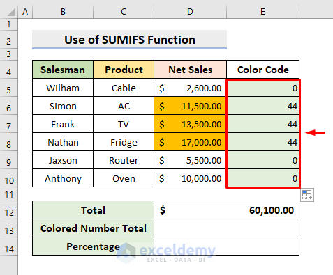
- Select cell D12 and enter the formula:
=SUM(D5:D10)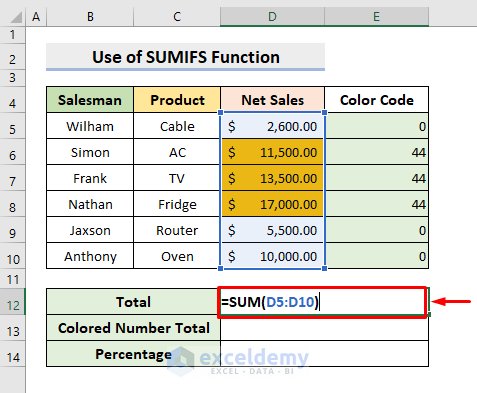
- Press Enter.
- Select cell D13 and enter the formula:
=SUMIFS(D5:D10,E5:E10,E6)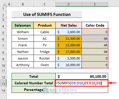
Here, D5:D10 is the sum range, E5:E10 is the criteria range and E6 is the criteria.
- Press Enter.
- Select cell D14 and type the formula:
=D13/D12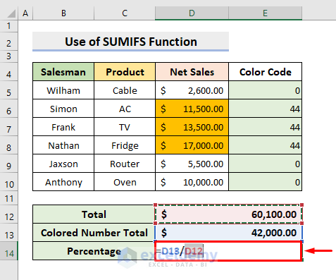
- Press Enter and select the ‘%’ icon in the Number group under the Home tab.

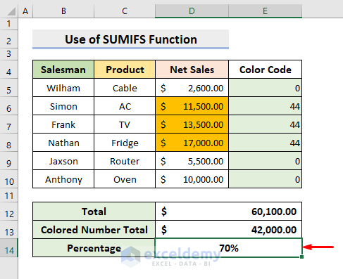
The precise percentage value will appear in cell D14:
Method 4 – Using Excel VBA
STEPS:
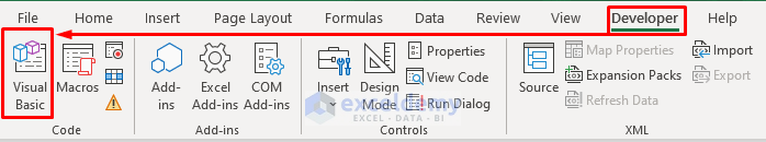
- Select Visual Basic under the Developer tab.
A new window will pop out.
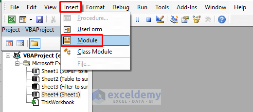
- Select Module under the Insert tab.
As a result, another window will pop out.
- There, paste the code given below:
Function ColorTotal(CClr As Range, rRng As Range)
Dim sum As Long
Dim color As Integer
color = CClr.Interior.ColorIndex
For Each cl In rRng
If cl.Interior.ColorIndex = color Then
sum = WorksheetFunction.sum(cl, sum)
End If
Next cl
ColorTotal = sum
End Function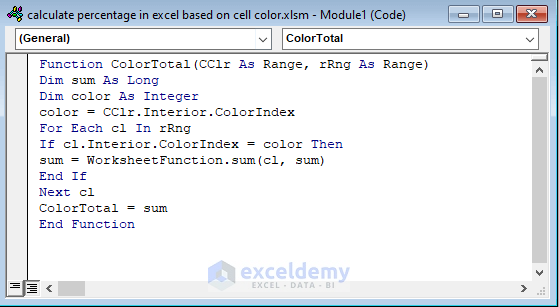
- Close the Visual Basic window.
- Select cell D12 and enter the formula:
=SUM(D5:D11)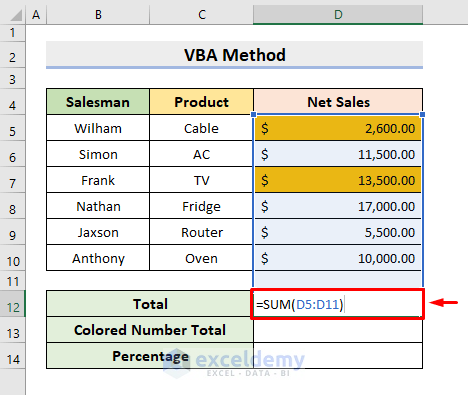
- Press Enter.
- Select cell D13 and enter the formula:
=ColorTotal(D5,D5:D10)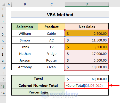
- Press Enter.
- Select cell D14 and enter the formula:
=D13/D12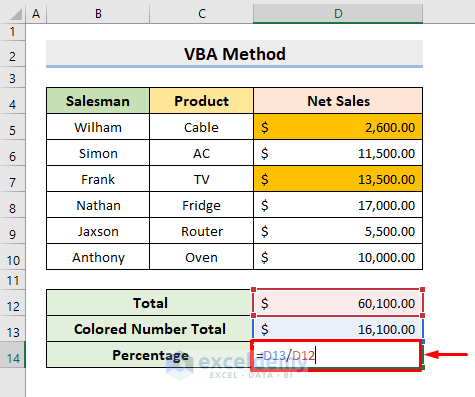
- Press Enter .
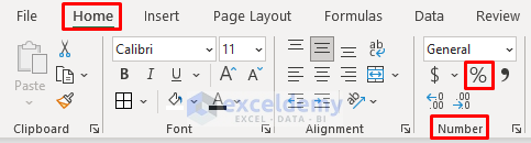
- Select the ‘%’ icon in the Number group under the Home tab.
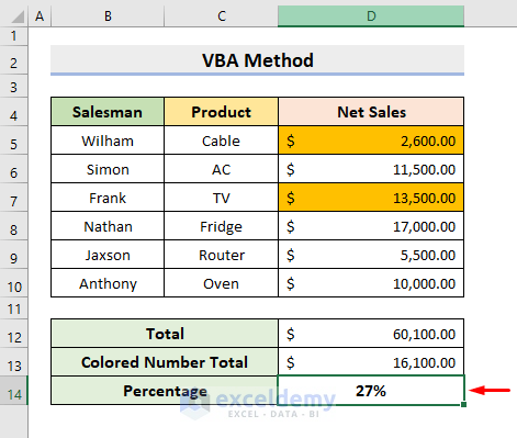
The percentage of the colored cells to the total net sales will appear in cell D14.
Read More: Calculate Percentage in Excel VBA
Download Practice Workbook
Related Articles
- How to Calculate Total Percentage from Multiple Percentages in Excel
- How to Calculate Percentage of Month in Excel
- How to Calculate Percentage of Percentage in Excel
- Percentage Showing as Thousand in Excel
- Why Are My Percentages Wrong in Excel?
- How to Remove Percentage in Excel
- How to Find the Percentage of Two Numbers in Excel
- How to Calculate Error Percentage in Excel
- How to Calculate Cumulative Percentage in Excel
<<Go Back to Calculate Percentage with Criteria in Excel | Calculating Percentages in Excel | How to Calculate in Excel | Learn Excel
Get FREE Advanced Excel Exercises with Solutions!
