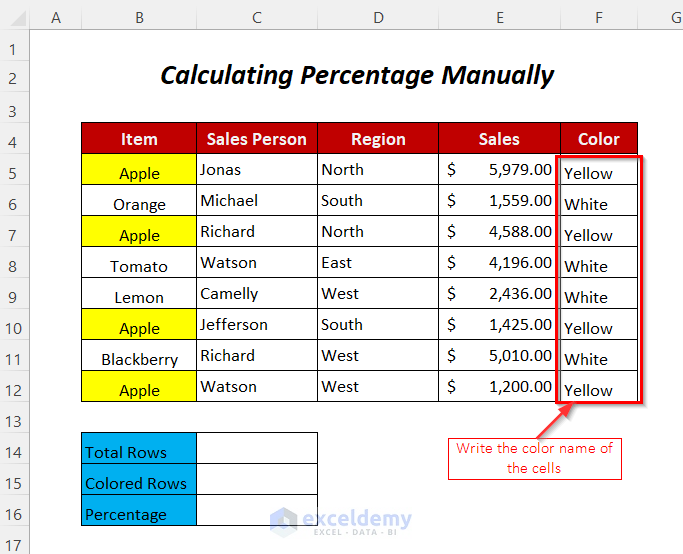
Method 1 – Calculate Percentages Based on Conditional Formatting Manually
Steps:
- Put down the name of the background colors of the cells of the Item column.
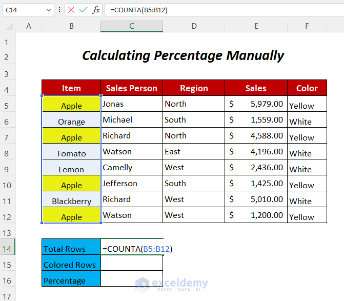
- Use the following formula in cell C14 for counting the total rows.
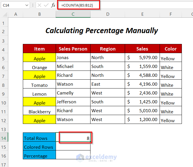
=COUNTA(B5:B12)B5:B12 is the range of the cells of the Item column and COUNTA will count the non-blank cells of this range.
- After pressing ENTER, you’ll have the number of total rows in this dataset.
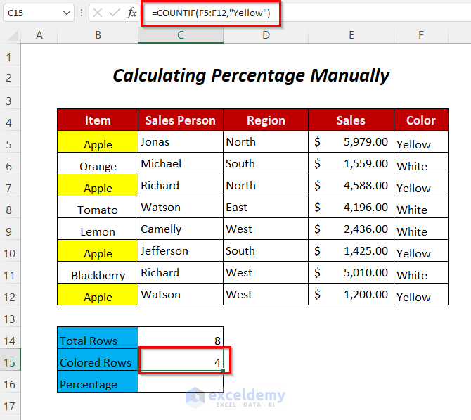
- Use the following formula in cell C15 for counting the colored cells
=COUNTIF(F5:F12, "Yellow")COUNTIF will give the number of cells with Yellow in the range F5:F12.

- Press ENTER. Get the number of highlighted cells as 4.
- To calculate the percentage, divide the Colored Rows by the Total Rows by using the following formula.
=C15/C14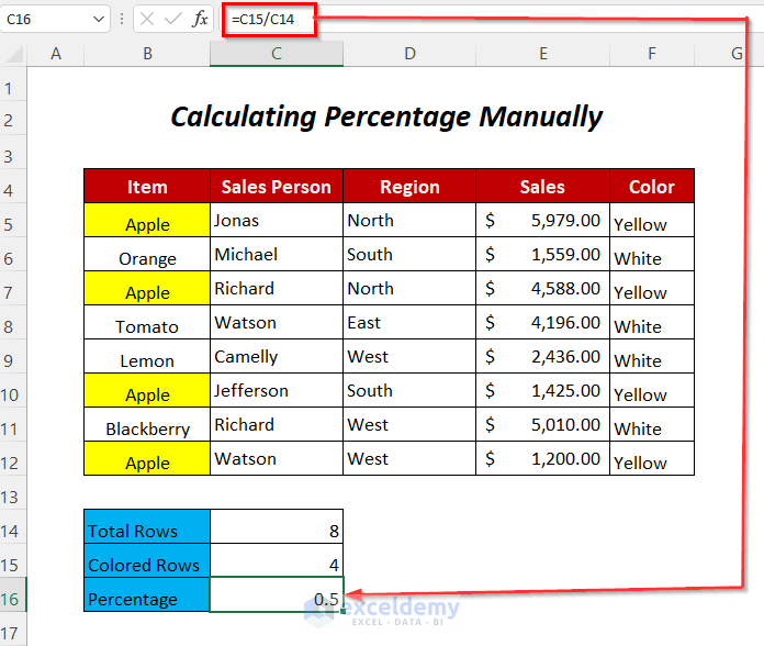
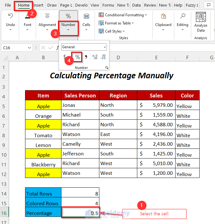
- To apply the Percentage form, select the value in cell C16 and go to Home Tab >> Number Group >> Percent Style Option.
You can also select it using the shortcut key CTRL+SHIFT+%.
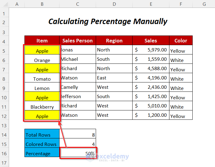
- You will get a percentage of 50% based on Conditional Formatting.
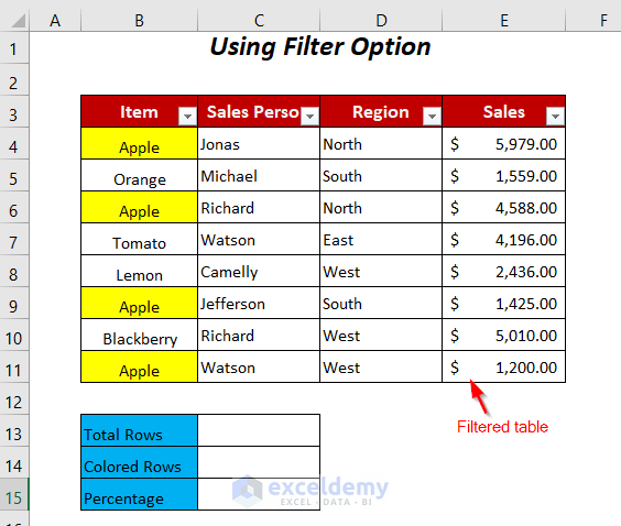
Method 2 – Calculate Percentages Based on Conditional Formatting Using the Filter Option
Steps:
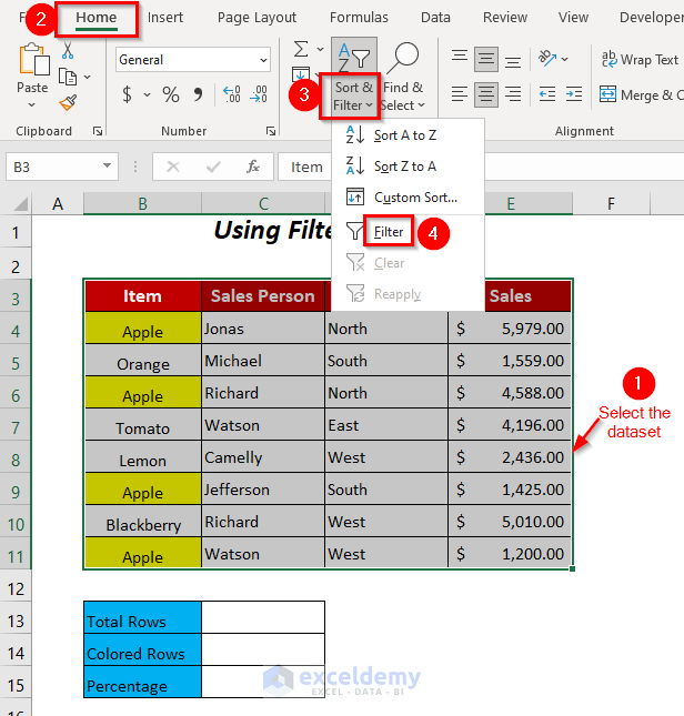
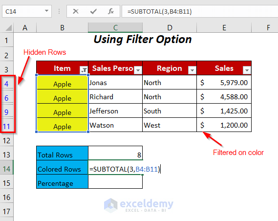
- Select the data range and go to Data Tab >> Sort & Filter Dropdown >> Filter Option.
- You will get the filter symbols on the dataset header row.
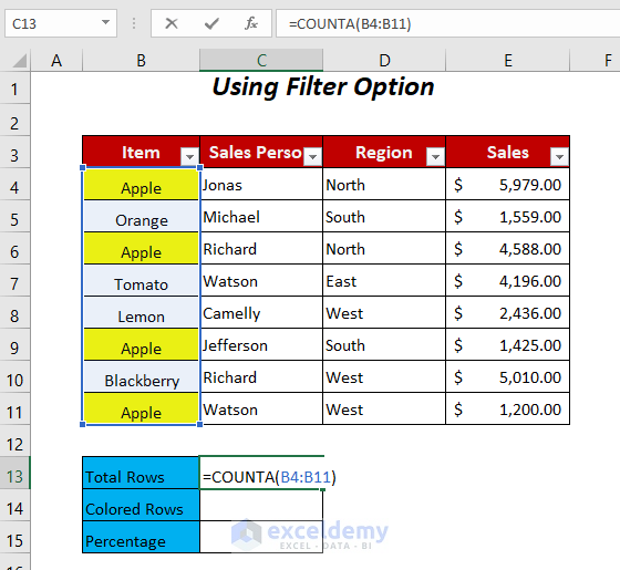
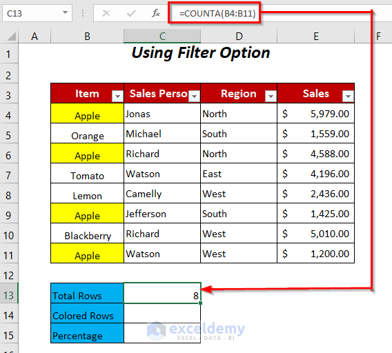
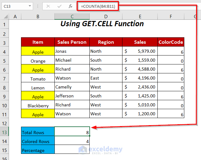
- Use the following formula in cell C13 for counting the total rows.
=COUNTA(B4:B11)B4:B11 is the range of the cells of the Item column, and COUNTA will count the non-blank cells in this range.
- You will get the number of total rows as 8.
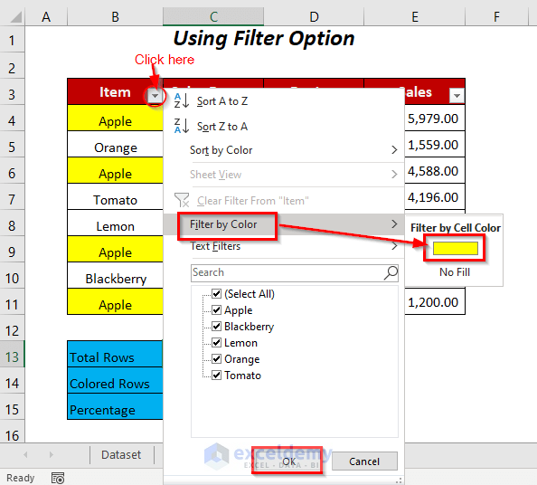
- Click on the dropdown sign in the Item column, select the Filter by Color option, and choose the Yellow color box from the Filter by Cell Color option.
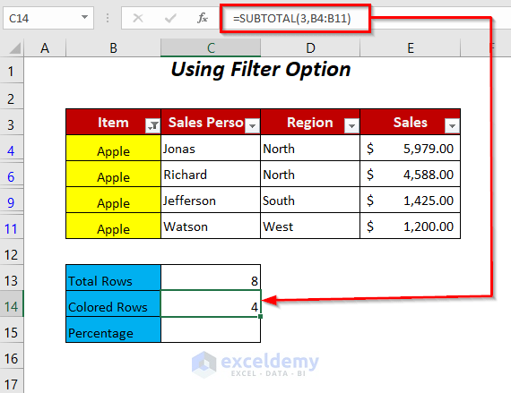
- Use the following formula in cell C14.
=SUBTOTAL(3,B4:B11)SUBTOTAL will count the number for only the unhidden cells 3 is for COUNTA function, and B4:B11 is the range of the Item column.
- We got the number of yellow color cells, which is 4.
- To get the percentage value, divide the Colored Rows by the Total Rows.
=C14/C13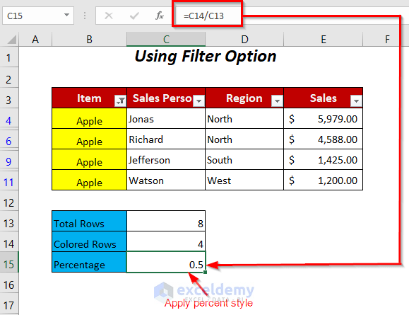
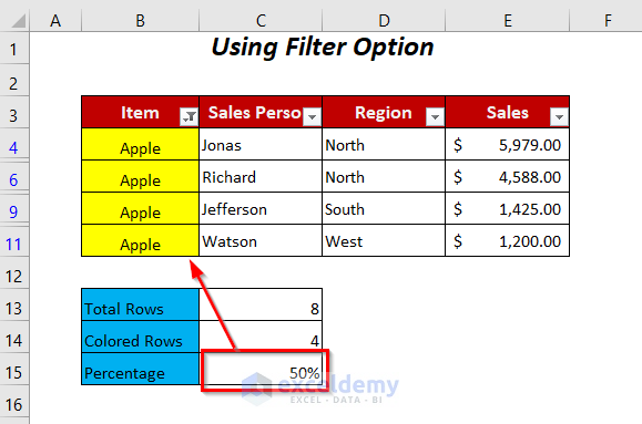
- After applying Percent Style, you’ll get the percentage of the highlighted cells.
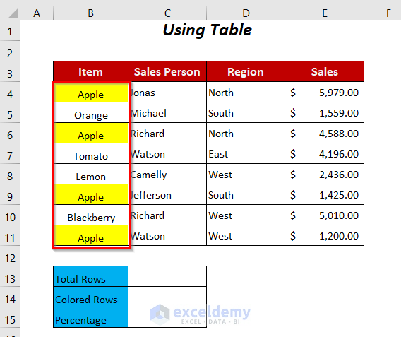
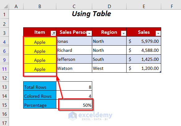
Method 3 – Calculate Percentages Based on Conditional Formatting Using a Table
We’ll use the same dataset as before.
Steps:
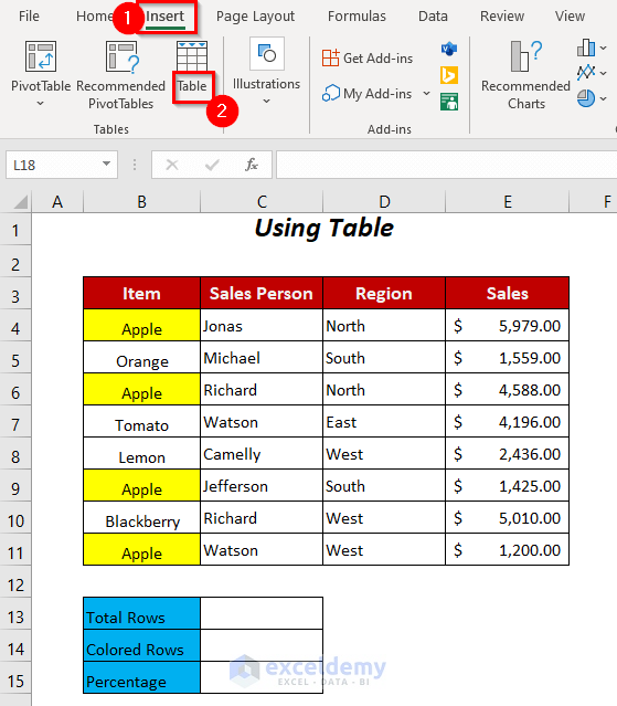
- Go to Insert tab and select the Table option.
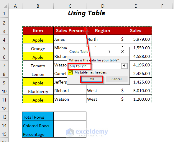
- The Create Table dialog box will appear.
- Select the range of your dataset.
- Check the My table has headers option and click OK.
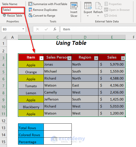
Excel will convert it into a table and name it.
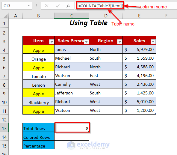
- Select cell C13 and use the formula
=COUNTA(B4:B11)B4:B11 is the range of the cells of the Item column and COUNTA will count the non-blank cells in this range.
- Excel will convert this automatically to the structured reference system and modify the formula as follows.
=COUNTA(Table3[Item])Table3 is the table name, and [Item] is the column name.
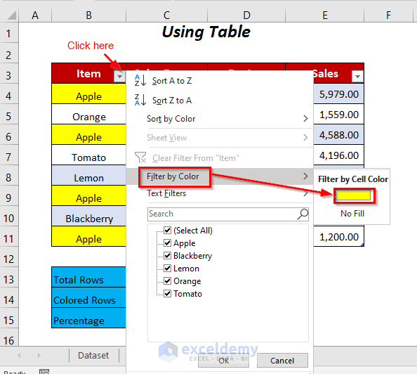
- Click on the dropdown sign in the Item column, select the Filter by Color option, and choose the Yellow color box from the Filter by Cell Color option.
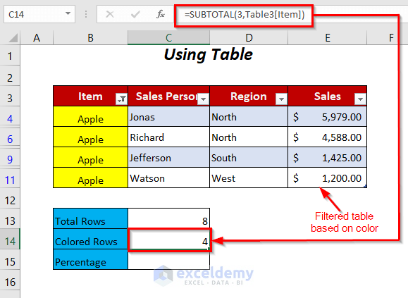
- Use the following formula in cell C14.
=SUBTOTAL(3,Table3[Item])SUBTOTAL will count the number for only the unhidden cells, 3 is for COUNTA function and Table3[Item] is the range of the Item column.
- To get the percentage value, divide the Colored Rows by the Total Rows.
=C14/C13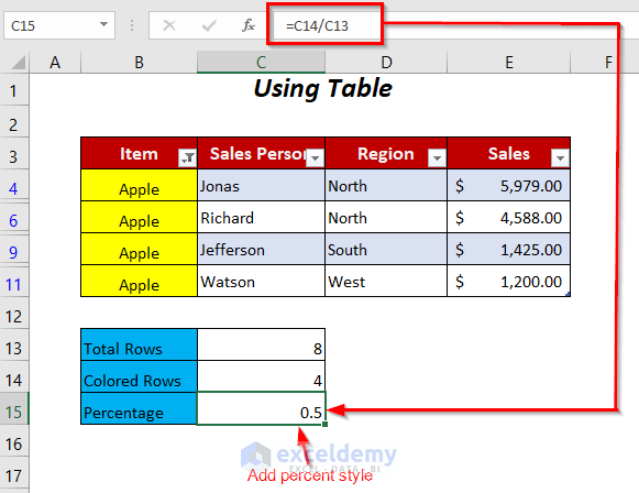
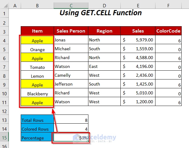
- After applying Percent Style, we’ll get the percentage of the highlighted cells as 50%.
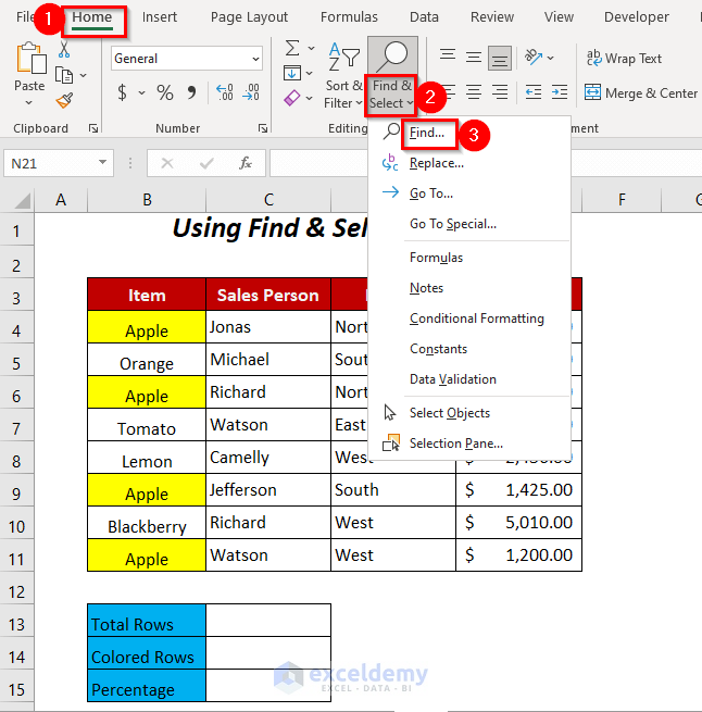
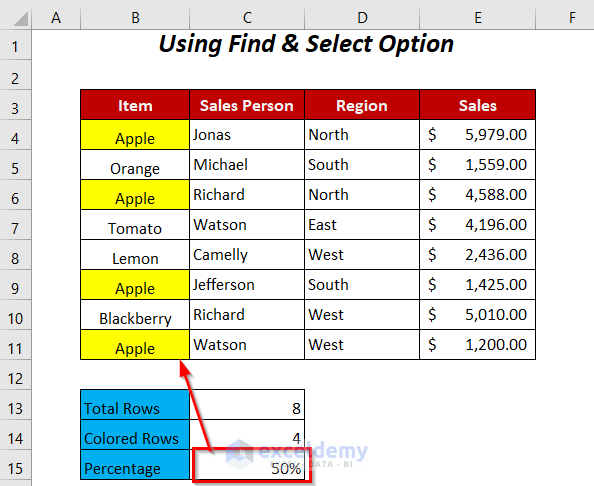
Method 4 – Calculate Percentages Based on Conditional Formatting Using Find & Select
Steps:
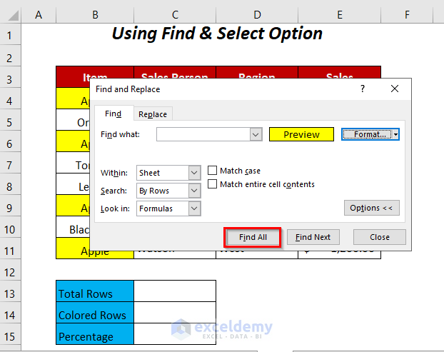
- Go to Home Tab >> Editing Group >> Find & Select Dropdown >> Find Option.
- The Find and Replace Dialog Box will pop up.
- Select the Format Option.
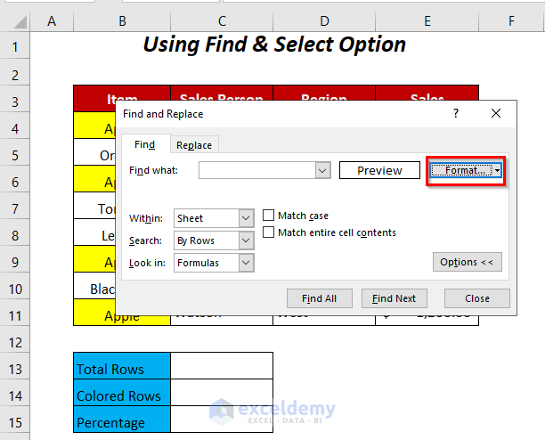
- The Find Format Dialog Box will appear.
- Select the Fill tab, choose the Yellow Color, and press OK.
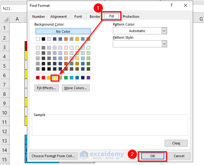
You will get a Preview section.
- Click the Find All option.
- You will see the number of yellow color cells, which is 4, in the bottom-left corner of the dialog box.
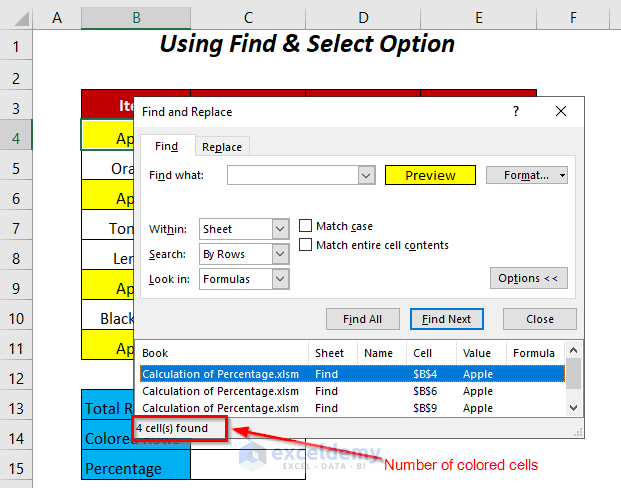
- Input that number in cell C14.
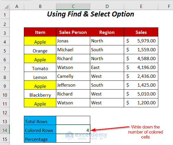
- To calculate the total number of rows, use the following formula in cell C13.
=COUNTA(B4:B11)B4:B11 is the range of the cells of the Item column and COUNTA will count the non-blank cells in this range.

- Calculate the percentage by dividing the Colored Rows by the Total Rows.
=C14/C13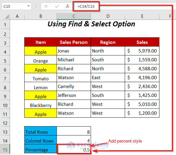
- After adding the Percent Style to this fraction number, you will get the percentage of Apples among other Items.
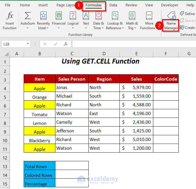
Method 5 – Calculate Percentages Based on Conditional Formatting Using the GET.CELL Function
Steps:
- Go to the Formulas tab >> Name Manager Option.
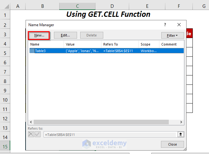
The Name Manager Wizard will appear.
- Select the New Option.
The New Name Dialog Box will pop up.
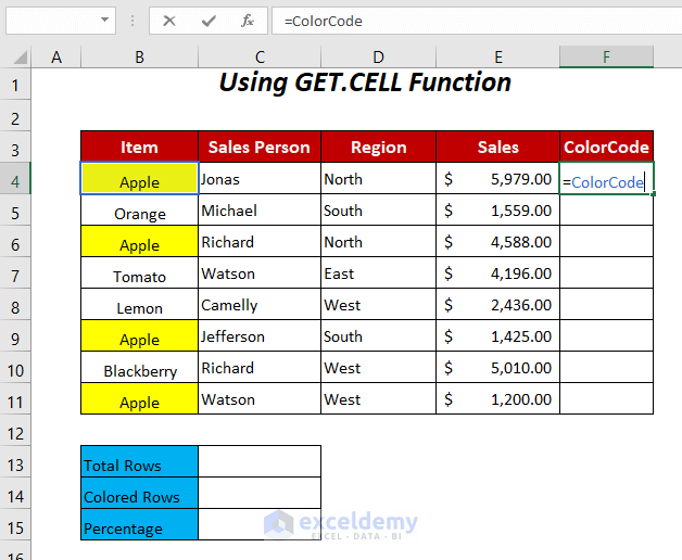
- Type any name in the Name Box. We used ColorCode.
- Select the Workbook Option in the Scope box.
- Use the following formula in the Refers to box:
=GET.CELL(38,Function!$B4)38 will return the Color Code, and Function!$B4 is the first highlighted cell in the Function sheet.
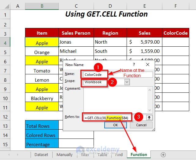
- Press OK.
- Use the created function name ColorCode in cell F4.
- Press Enter and drag down the Fill Handle Tool.
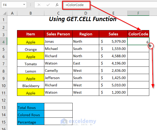
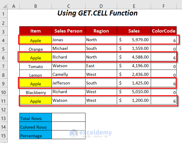
- We get the Color Code 6 for the yellow color cells of the Item column.
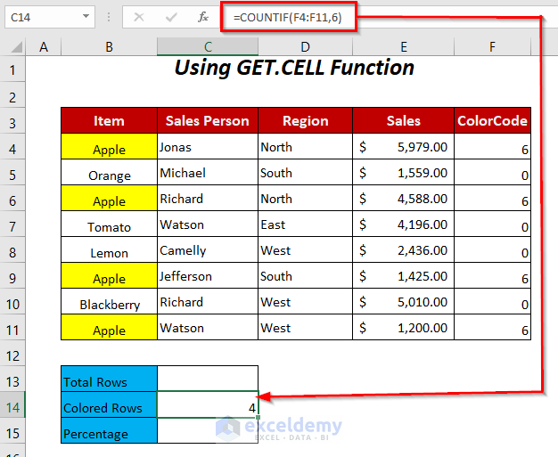
- Use the following formula in cell C14
=COUNTIF(F4:F11,6)COUNTIF will give the number of cells having 6 in the range F4:F11. This is the result of the previous formula.
- For the Total Rows, use the following formula in cell C13
=COUNTA(B4:B11)B4:B11 is the range of the cells of the Item column and COUNTA will count the non-blank cells in this range.
- To determine the percentage value, use the following formula in cell C15.
=C14/C13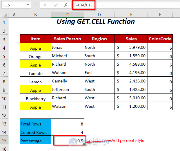
- After adding Percent Style, we will get the percentage based on Conditional Formatting.
Method 6 – Using VBA Code
Steps:
- Go to Developer Tab >> Visual Basic Option.
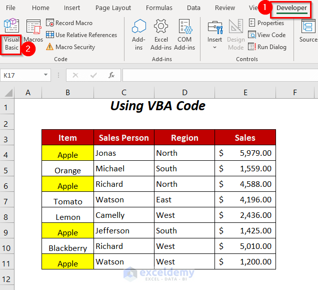
- The Visual Basic Editor will open.
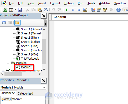
- Go to Insert Tab >> Module Option.
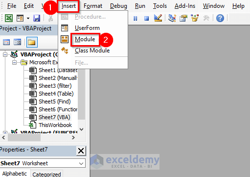
A Module will be created.
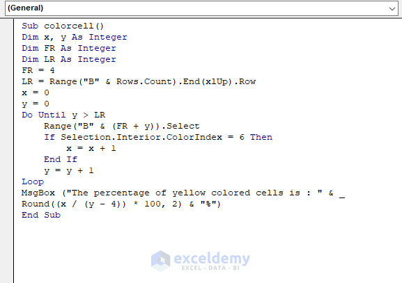
- Insert the following code
Sub colorcell()
Dim x, y As Integer
Dim FR As Integer
Dim LR As Integer
FR = 4
LR = Range("B" & Rows.Count).End(xlUp).Row
x = 0
y = 0
Do Until y > LR
  Range("B" & (FR + y)).Select
    If Selection.Interior.ColorIndex = 6 Then
       x = x + 1
    End If
    y = y + 1
Loop
MsgBox ("The percentage of yellow colored cells is : " & _
Round((x / (y - 4)) * 100, 2) & "%")
End Sub
We declared x, y, FR, LR as Integer, we have assigned FR to 4 which is the starting row of our dataset and LR will determine the last row of the dataset.
DO UNTIL loop will count the colored cells for each cell of Column B, and the VBA IF Statement will identify if the color of the cell is yellow ( color code = 6 ) for these cells, x will be increased by 1, and using the formula Round((x / (y – 4)) * 100, 2) we will get the percentage value rounded up to 2 values after the decimal point. y – 4 will give the total rows, and here, you have to subtract the first-row number from y.
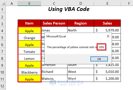
- Press F5. You will get the percentage based on Conditional Formatting in a message box (MsgBox).
Download the Workbook
Related Articles
- How to Calculate Percentage of Month in Excel
- How to Calculate Total Percentage from Multiple Percentages in Excel
- How to Calculate Percentage of Percentage in Excel
- Percentage Showing as Thousand in Excel
- Why Are My Percentages Wrong in Excel?
- How to Remove Percentage in Excel
- How to Find the Percentage of Two Numbers in Excel
- How to Calculate Error Percentage in Excel
- How to Calculate Cumulative Percentage in Excel
<<Go Back to Calculate Percentage with Criteria in Excel | Calculating Percentages in Excel | How to Calculate in Excel | Learn Excel
Get FREE Advanced Excel Exercises with Solutions!
