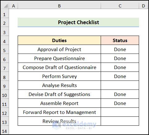
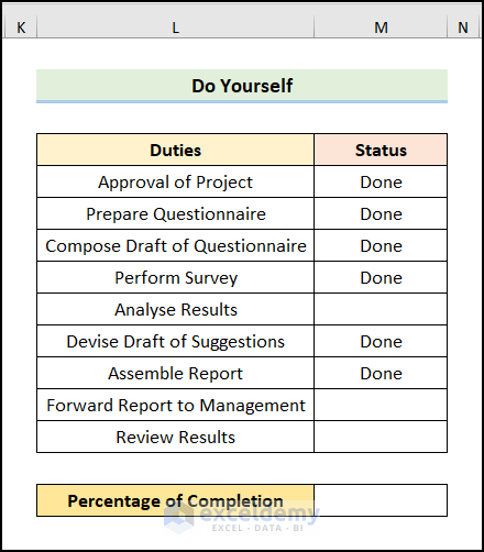
The sample dataset contains a Project Checklist with a list of Duties and a Status column. We will calculate the percentage of filled cells with the Done status.
Method 1 – Using COUNTA Function
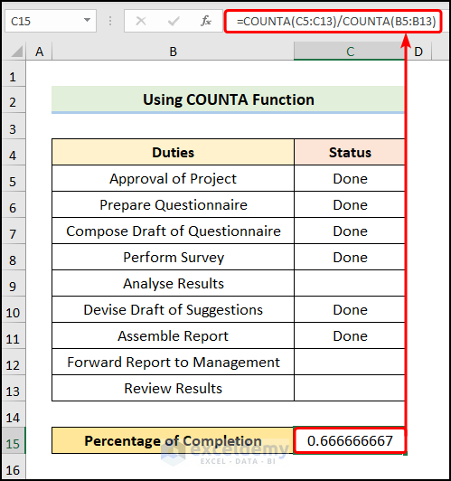
The COUNTA function will count the number of non-blank and the total number of cells in the given range and return the percentage of filled cells.
Steps:
- Enter the formula below.
=COUNTA(C5:C13)/COUNTA(B5:B13)
The B5:B13 and C5:C13 range of cells refer to the Duties and Status columns respectively.
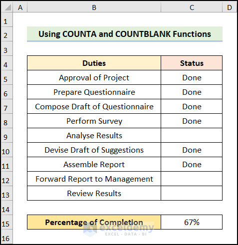
- Press the CTRL + SHIFT + % to format the values as a percentage. You can use the Percent Style button in the Number ribbon group from the Home tab.
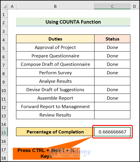
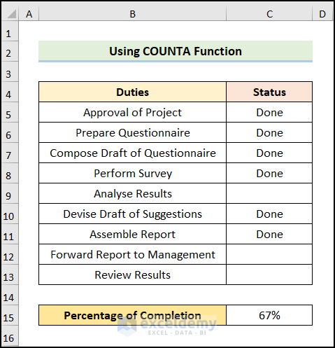
The results should look like the below image.
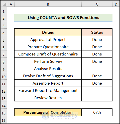
Method 2 – Using COUNTA and ROWS Functions
Steps:
- Type the below formula in the relevant cell.
=COUNTA(C5:C13)/ROWS(C5:C13)
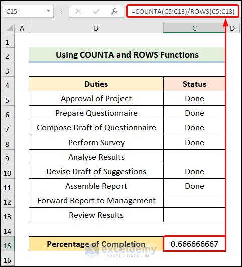
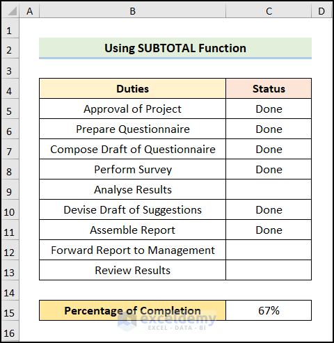
- Press the CTRL + SHIFT + % keys to apply percentage formatting.
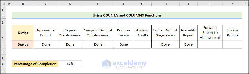
Method 3 – Utilizing COUNTA and COLUMNS Functions
Steps:
- Navigate to the D8 cell and insert the below formula in the Formula Bar.
=COUNTA(C5:K5)/COLUMNS(C5:K5)
The C5:K5 cells point to the Status row.
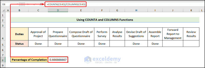
- Press the CTRL + SHIFT + % keys to apply percentage formatting.
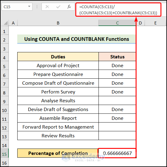
Method 4 – Applying COUNTA and COUNTBLANK Functions
The COUNTBLANK function counts the number of empty cells within a selected range.
Steps:
- Type the below formula in the relevant cell.
=COUNTA(C5:C13)/(COUNTA(C5:C13)+COUNTBLANK(C5:C13))
Read More: How to Apply Percentage Formula for Multiple Cells in Excel
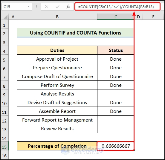
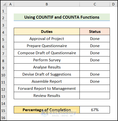
Method 5 – Combining COUNTIF and COUNTA Functions
Steps:
- Type the below formula in the relevant cell.
=COUNTIF(C5:C13,"<>")/COUNTA(B5:B13)
Read More: How to Add Percentage to Price with Excel Formula
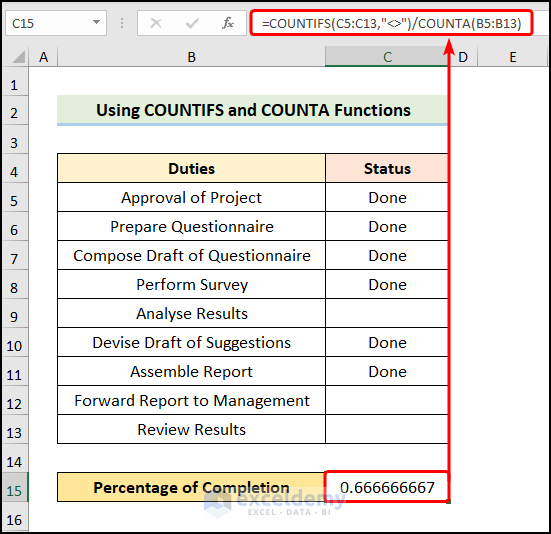
Method 6 – Employing COUNTIFS and COUNTA Functions
Steps:
- Type the below formula in the relevant cell.
=COUNTIFS(C5:C13,"<>")/COUNTA(B5:B13)

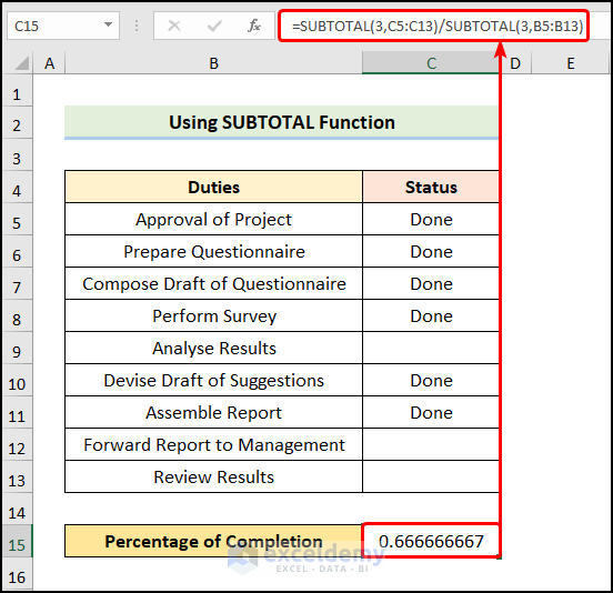
Method 7 – Using SUBTOTAL Function
Steps:
- Type the below formula in the relevant cell.
=SUBTOTAL(3,C5:C13)/SUBTOTAL(3,B5:B13)
Related Articles
- Calculate Percentage Using Absolute Cell Reference in Excel
- Calculate Percentage in Excel VBA
- How to Calculate Percentage above Average in Excel
- How to Apply Percentage Formula in Excel for Marksheet
- IF Percentage Formula in Excel
- How to Calculate Contribution Percentage with Formula in Excel
- How to Use Food Cost Percentage Formula in Excel
- How to Calculate Percentage for Multiple Rows in Excel
- How to Calculate Variance Percentage in Excel
<<Go Back to Calculate Percentage with Criteria in Excel | Calculating Percentages in Excel | How to Calculate in Excel | Learn Excel
Get FREE Advanced Excel Exercises with Solutions!
