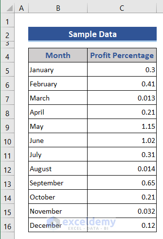
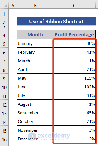
We will consider a simple dataset which contains profits for each month in decimal form. We need to convert that into percentile.
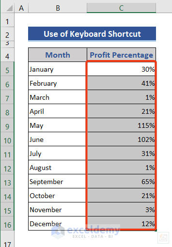
Method 1 – Using the Keyboard Shortcut
Steps:
- Select the range C5:C16.
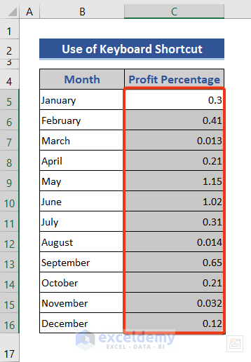
- Press Ctrl + Shift + %.
Read More: How to Divide a Value to Get a Percentage in Excel
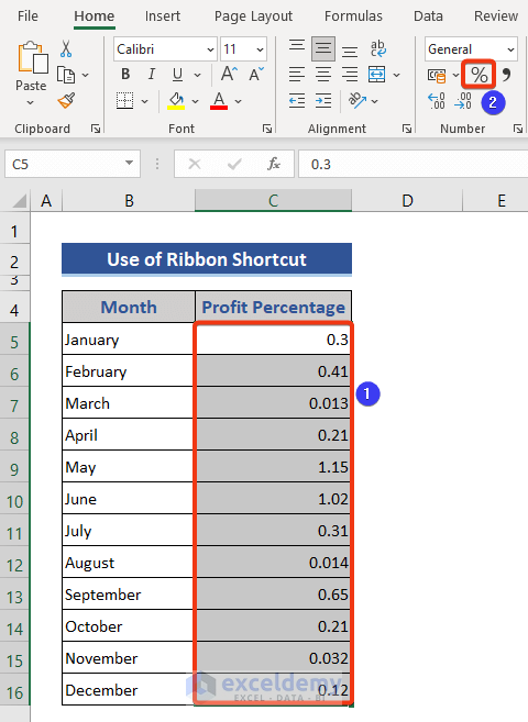
Method 2 – Using the % Button from the Ribbon
Steps:
- Select the data range.
- Click on the Percentage symbol in the Number group.
- Here are the results.
- Select the dataset.
- Click on the Increase Decimal option from the Number group.
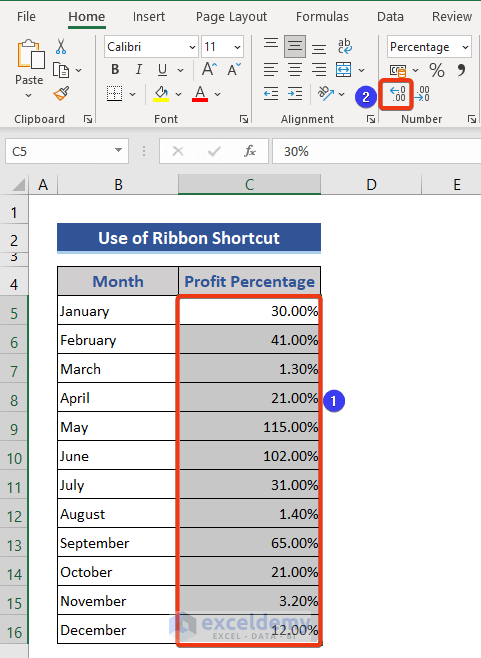
- We can see more decimal points for increased accuracy.
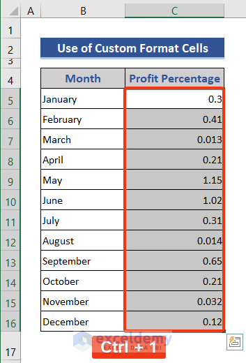
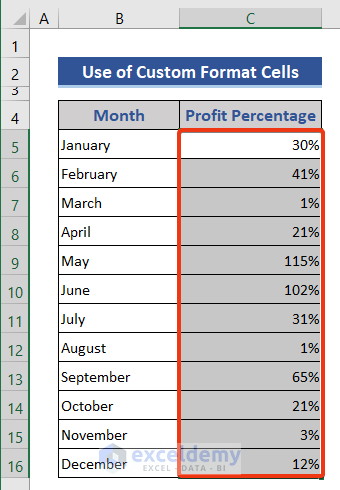
Method 3 – Applying a Custom Format
Steps:
- Select the data range.
- Press Ctrl + 1 to get the Format Cells window.
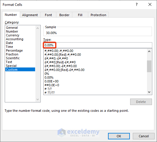
- Choose the Custom option from the Number tab.
- Input 0% in the Type section.
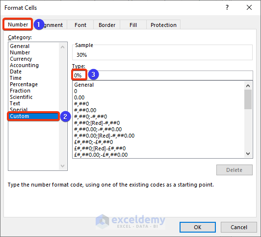
- Press the OK button.
- Enter the Format Cells window.
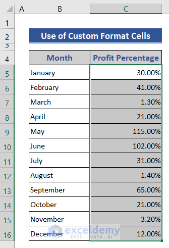
- Change the Type to 0.00%.
- Here are the results.
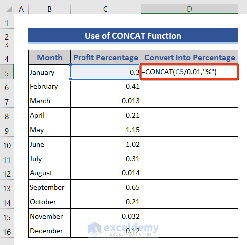
Method 4 – Using the CONCAT Function to Convert Numbers into Percentages
The CONCAT function is the updated form of the CONCATENATE function.
Steps:
- Add a new column on the right to show the result.
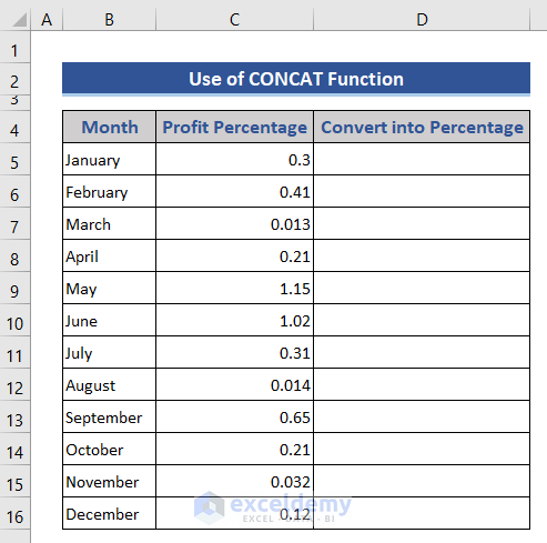
- Put the following formula in Cell D5.
=CONCAT(C5/0.01,"%")
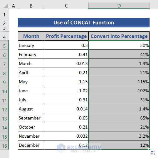
- Press the Enter button and drag the Fill Handle icon.
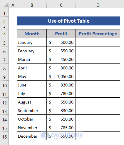
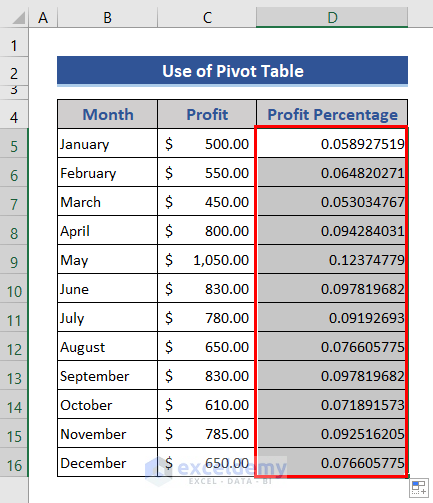
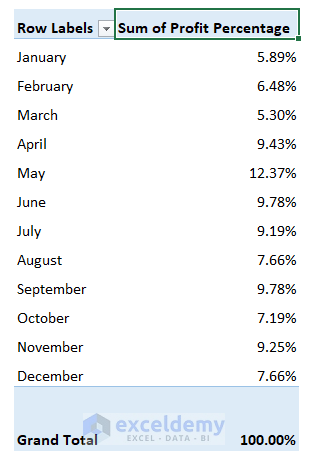
Method 5 – Convert Numbers to Percentages in an Excel Pivot Table
We have a dataset of each month’s profit of 2021 of a super shop. We will calculate the profit percentage for each month based on the total profit of the year.
Steps:
- Put the following formula in Cell D5.
=C5/SUM($C$5:$C$16)
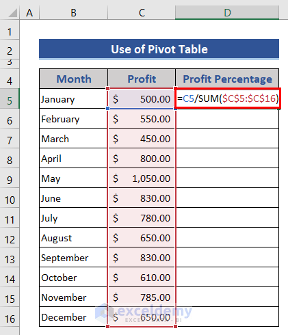
- Press the Enter button and drag the Fill Handle icon.
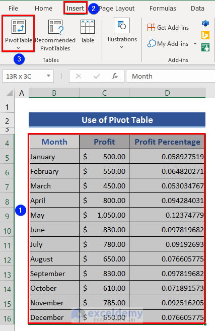
- Select the whole dataset.
- Click on the Pivot Table option from the Insert tab.
- A new window appears.
- Choose the Existing Worksheet option to place the Pivot table.
- Select a cell in the worksheet for the Location section.
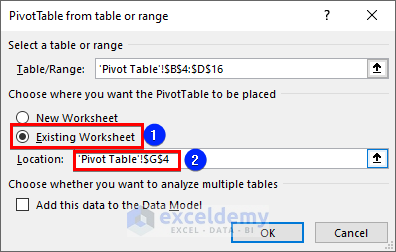
- Press the OK button.
- The PivotTable Fields section appears.
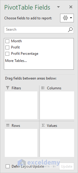
- Tick the Month option and place it in the Rows field.
- Tick the Profit Percentage option and place it in the Values field.
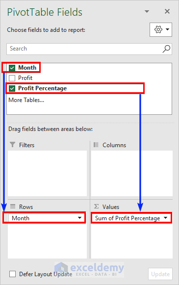
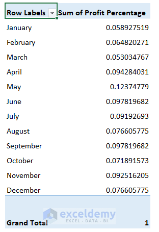
- The results are in decimal form.
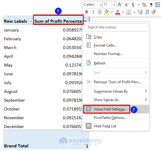
- Go to the Sum of Profit Percentage cell and right-click.
- Choose Value Field Settings from the Context Menu.
- The Value Filed Settings window appears.
- Choose the Show Values As option.
- Click on the drop-down.
- Choose the % of Column Total option.
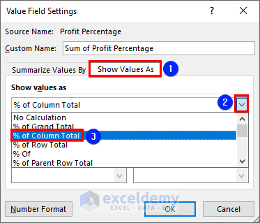
- Press the OK button.
How Do I Remove the Percentage Symbol in Excel Without Changing Values?
We have the following dataset. We’ll change the percentages to numbers without the percentage sign, but keep their value (so 30% becomes 30).
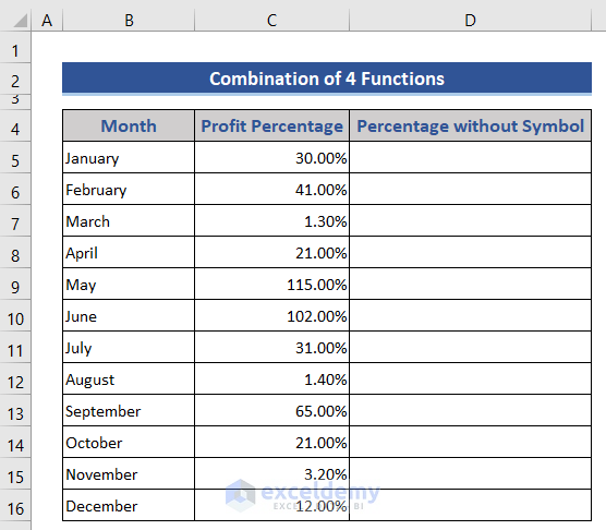
Steps:
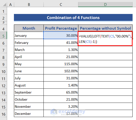
- Go to Cell D5 and insert the following formula.
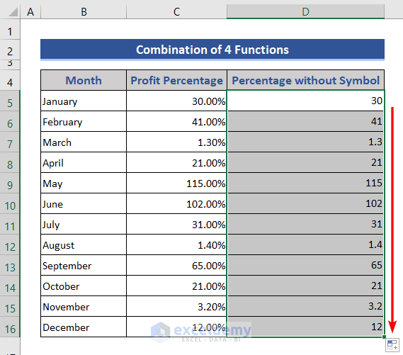
=VALUE(LEFT(TEXT(C5,"00.00%"),LEN(C5)-1))
- Press the Enter button and drag the Fill Handle icon.
Formula Breakdown:
- TEXT(C5,”00.00%”)
This converts any value in the given format in the formula.
Result: 30.00%
- LEN(C5)
This defines the length of Cell C5.
Result: 3
- LEFT(TEXT(C5,”00.00%”),LEN(C5)-1)
This returns characters from the start. How many digits will appear depends on the LEN function.
Result: 30
- VALUE(LEFT(TEXT(C5,”00.00%”),LEN(C5)-1))
The VALUE function converts text strings into numbers.
Result: 30
Download the Practice Workbook
Related Articles
- How to Calculate Percentage of Total in Excel
- How to Convert Number to Percentage in Excel
- How to Calculate Reverse Percentage in Excel
- How to Find the Percentage of Two Numbers in Excel
- How to Convert Percentage to Number in Excel
- How to Convert Percentage to Whole Number in Excel
- How to Show One Number as a Percentage of Another in Excel
- How to Add a Percentage to a Number in Excel
- Make an Excel Spreadsheet Automatically Calculate Percentage
<<Go Back to Calculating Percentages in Excel | How to Calculate in Excel | Learn Excel
Get FREE Advanced Excel Exercises with Solutions!
