Method 1 – Utilizing Percent Style Button
Step 01: Calculate Fraction of Discount
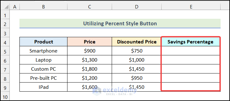
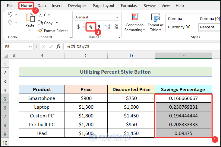
- Create a new column named Savings Percentage, as shown in the following image.
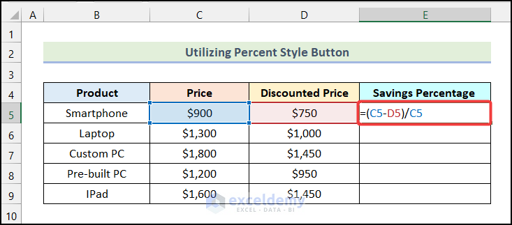
- Enter the following formula in cell E5.
=(C5-D5)/C5Cell C5 refers to the cell of the Price column, and cell D5 indicates the cell of the Discounted Price column.
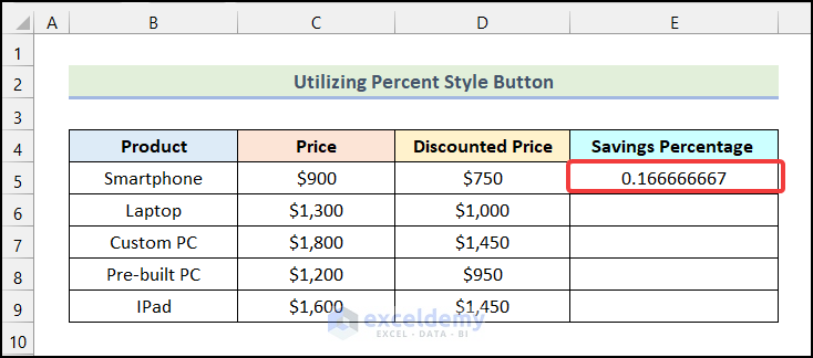
- Press ENTER.
A fraction of the discount for Smartphone will be available on your worksheet.
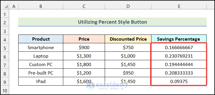
- Use the AutoFill option of Excel to get the rest of the outputs.
Step 02: Convert to Percentage Format
- Select the cells of the “Savings Percentage” column.
- Go to the Home tab from Ribbon.
- Click on the Percentage Style option from the Number group.
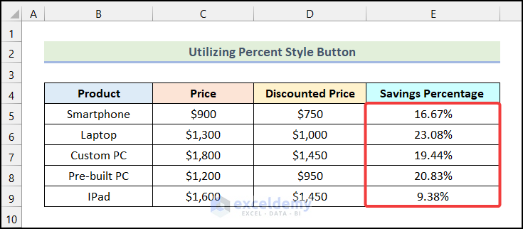
You will have the savings percentages for various “Products” as marked in the following picture.
Method 2 – Applying Keyboard Shortcut
Steps:
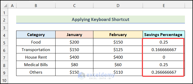
- Follow the procedures mentioned in Step 01 of the 1st method to get the following output.
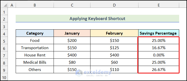
- Select the cells of the “Savings Percentage” column and press the keyboard shortcut CTRL + SHIFT + %.
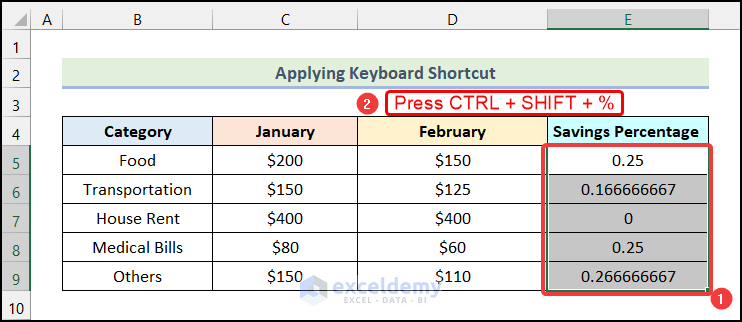
Your savings percentages will be available as demonstrated in the image below.
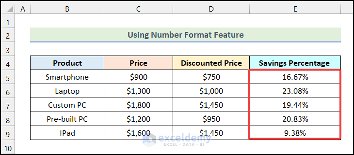
Method 3 – Using Number Format Feature
Steps:
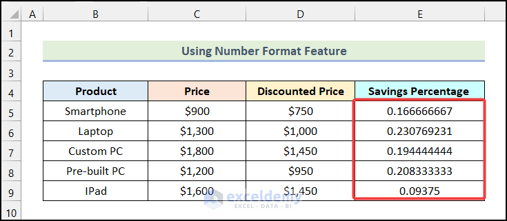
- Follow the steps used in Step 01 of the 1st method and you will have the following outputs as marked below.
- Select the cells of the “Savings Percentage” column and go to the Home tab.
- Click on the Number Format option from the Number ribbon group.
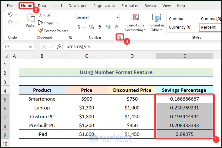
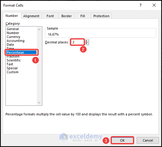
The Format Cells dialogue box will open on your worksheet.
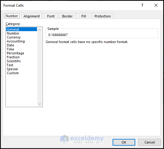
Note: You can also use the keyboard shortcut CTRL + 1 to open the Format Cells dialogue box directly.
- In the Format Cells dialogue box, choose the Percentage option.
- Add the number of decimal places you want in the percentage format by clicking the increase and decrease buttons.
- Click OK.
You will have the savings percentage as demonstrated in the following picture.
How to Calculate Cost Percentage in Excel
Steps:
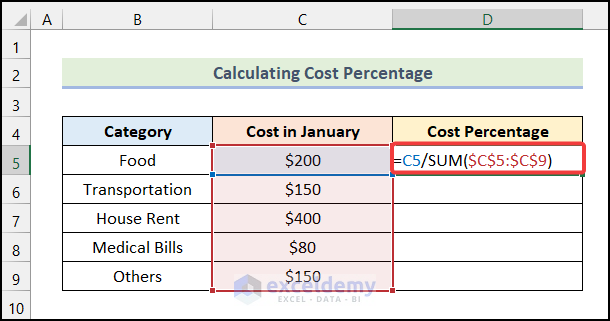
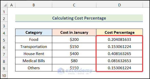
- Use the following in cell D5.
=C5/SUM($C$5:$C$9)Cell C5 refers to the cost of “Food” in January month, and the SUM function will return the summation of the range of cells $C$5:$C$9.
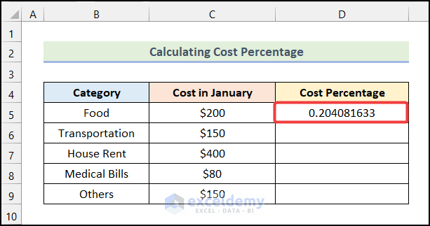
- Hit ENTER.
You will have the following output in cell D5, as marked in the image below.
- Use the AutoFill feature of Excel to have the remaining outputs.
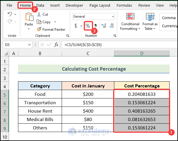
- Select the cells of the “Cost Percentage” column.
- Go to the Home tab from Ribbon.
- Click on the Percentage Style button.
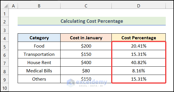
You will have the cost percentages against each “Category” as shown in the image below.
Download Practice Workbook
Related Articles
- How to Calculate Error Percentage in Excel
- How to Calculate Cumulative Percentage in Excel
- How to Calculate Remaining Shelf Life Percentage in Excel
- How to Calculate Percentage of Completion in Excel
- How to Calculate Absenteeism Percentage in Excel
- How to Calculate Productivity Percentage in Excel
- How to Calculate Variance Percentage in Excel
- How to Calculate Accuracy Percentage in Excel
- How to Calculate Grade Percentage in Excel
- How to Calculate Win-Loss Percentage in Excel
- How to Calculate SLA Percentage in Excel
- How to Calculate Percentage of Budget Spent in Excel
- How to Calculate Utilization Percentage in Excel
<< Go Back to Calculating Percentages | Calculate in Excel | Learn Excel
Get FREE Advanced Excel Exercises with Solutions!
