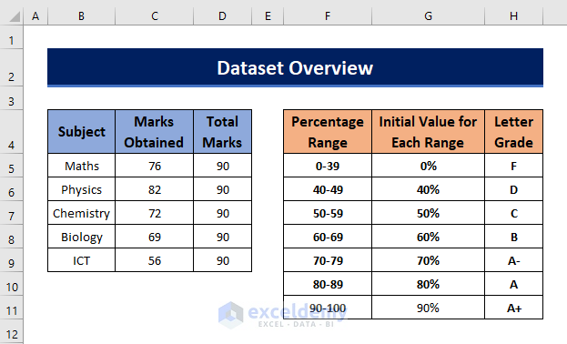
We have a grade sheet of a student with obtained marks in five distinct subjects. We want to calculate the grade percentage considering the letter grading system and the grading sheet.
Method 1 – Using the VLOOKUP Function to Calculate the Grade Percentage
VLOOKUP function looks for a lookup value or a range of lookup values in the leftmost column of a defined lookup array and then returns a specific value from the index column number of the lookup array based on the exact or partial match.
The syntax of the VLOOKUP function is:
VLOOKUP(lookup_value,table_array,col_index_num,[range_lookup])Part 1.1 – Getting the Letter Grade and Percentage for Each Subject Separately
Steps
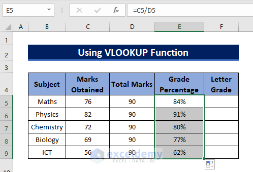
- Insert the following function in E5.
=C5/D5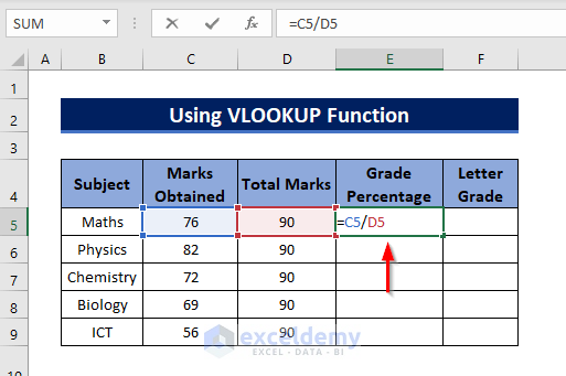
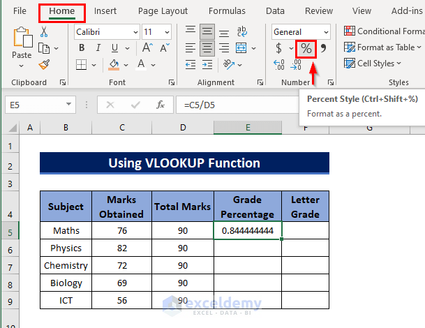
- Press Enter and you will get the result in decimal format.
- Click the Percent Style icon in the Number group of the Home tab.
- Select the Fill Handle tool and drag it down to Autofill the formula.
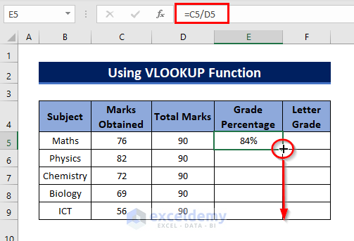
- You’ll get grade percentages for all subjects.
- We moved the grading table to the range D12:E18.
- Use the formula below in F5.
=VLOOKUP(E5,$D$12:$E$18,2,TRUE)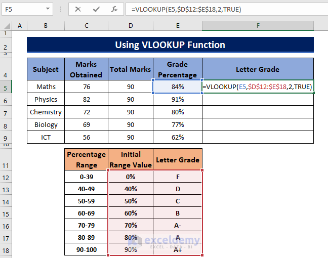
The formula locks in the search array reference with the dollar signs ($) to make it into an absolute reference. This allows that part of the formula to stay when copying the formula to other rows or columns.
- Press Enter.
Formula Unlocking
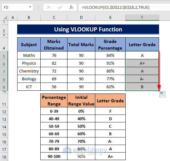
The VLOOKUP function looks for the cell value of E5 (84%) in the lookup array $D$12:$E$18.
After finding the value in the specified range of the array, it takes the value of the second column (as we have defined column index 2) for an approximate match (argument: TRUE) of that array in the same row of the lookup value and returns the result in the selected cell.
Output=> A.
- Drag the formula down and the letter grades for all subjects will be shown.
Read More: Make an Excel Spreadsheet Automatically Calculate Percentage
Part 1.2 – Calculating the Average Grade Percentage and Average Letter Grade in Excel
Steps
- Add two extra columns named Average Grade Percentage and Average Letter Grade to the previous data set.
- Apply the AVERAGE function to calculate the average letter grade of all the subjects.
=AVERAGE(E5:E9)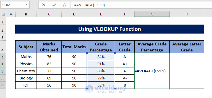
- Apply the VLOOKUP function to find the Average Letter Grade:
=VLOOKUP(G5,D12:E18,2,TRUE)Method 2 – Using a Nested IF Formula to Calculate the Grade Percentage in Excel
Steps
- Select F5 and apply the following formula to create a condition to find the letter grade:
=IF(E5<40%, $E$12, IF(E5<50%, $E$13, IF(E5<60%, $E$14, IF(E5<70%, $E$15, IF(E5<80%, $E$16, IF(E5<90%, $E$17, $E$18))))))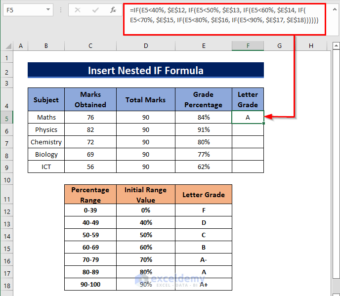
Formula Unlocking
We’re using the Nested IF function to add multiple conditions to meet our criteria.
If the value in Cell E5 does not meet the first condition, it’ll go to the next IF, and so on. Once this process fulfills the condition for E5, the fixed Letter Grade from the cells (E12:E18) will be assigned to it.
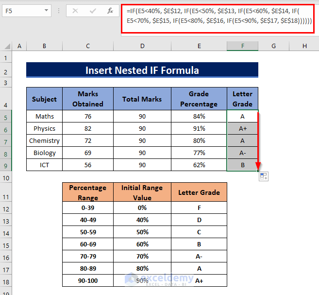
- Drag the formula for the other cells and you’ll get the expected results.
Read More: How to Calculate Cumulative Percentage in Excel
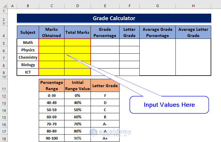
Grade Percentage Calculator
We are providing a grade percentage calculator in the Excel file. Input the values in the marked area and this calculator will automatically calculate the grade percentage and show you the letter grade.
Download the Calculator
Related Articles
- How to Calculate Win-Loss Percentage in Excel
- How to Calculate SLA Percentage in Excel
- How to Calculate Error Percentage in Excel
- How to Calculate Remaining Shelf Life Percentage in Excel
- How to Calculate Percentage of Completion in Excel
- How to Calculate Percentage of Budget Spent in Excel
- How to Calculate Utilization Percentage in Excel
- How to Calculate Absenteeism Percentage in Excel
- How to Calculate Savings Percentage in Excel
- How to Calculate Productivity Percentage in Excel
- How to Calculate Variance Percentage in Excel
- How to Calculate Accuracy Percentage in Excel
<< Go Back to Calculating Percentages | Calculate in Excel | Learn Excel
Get FREE Advanced Excel Exercises with Solutions!
