Download Practice Workbook
Download this practice workbook to exercise.
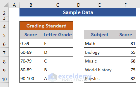
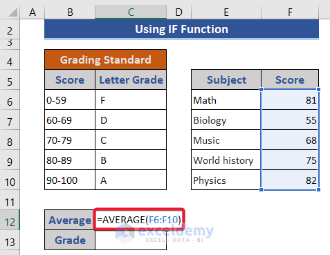
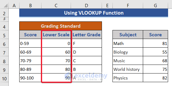
A sample letter grade standard is shown in the dataset below.
Method 1 – Use the IF and the AVERAGE Functions to Calculate Average Letter Grades
The IF function checks whether a condition is met and, returns a value if True and another if False.
The AVERAGE function returns the average (arithmetic mean) of its arguments.
Steps:
- Add two new rows to the sheet.
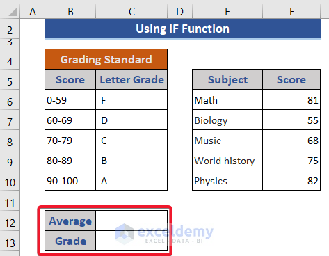
- Calculate the average score in C12.
- Enter the following formula.
=AVERAGE(F6:F10)
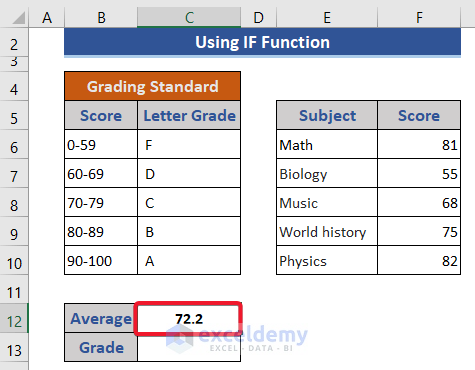
- Press Enter to see the result.
- Enter another formula in C13.
=IF(C12>=90,"A",IF(C12>=80,"B",IF(C12>=70,"C",IF(C12>=60,"D","F"))))
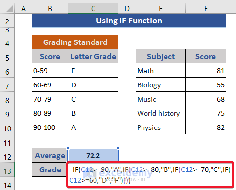
- Press Enter.
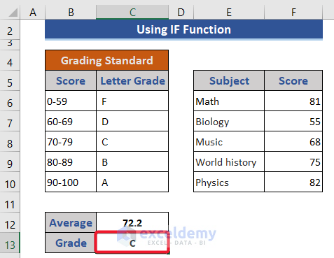
This is the output.
Read More: How to Make Result Sheet in Excel (with Easy Steps)
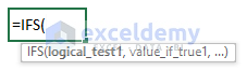
Method 2 – Apply the IFS Function
The IFS function checks whether one or more conditions are met and, returns a value corresponding to the first TRUE condition.
Steps:
- Go to C13 and enter the formula.
=IFS(C12>=90,"A",C12>=80,"B",C12>=70,"C",C12>=60,"D",C12<60,"F")
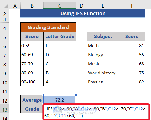
- Press Enter to see the result.
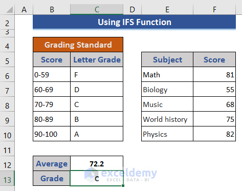
This is the output.
Read More: How to Make a Grade Calculator in Excel (2 Suitable Ways)
Similar Readings
- How to Calculate Final Grade in Excel (with Easy Steps)
- Calculate College GPA in Excel (3 Handy Approaches)
- How to Calculate Subject Wise Pass or Fail with Formula in Excel
- Make Automatic Marksheet in Excel (with Easy Steps)
- How to Calculate Grades with Weighted Percentages in Excel
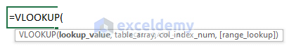
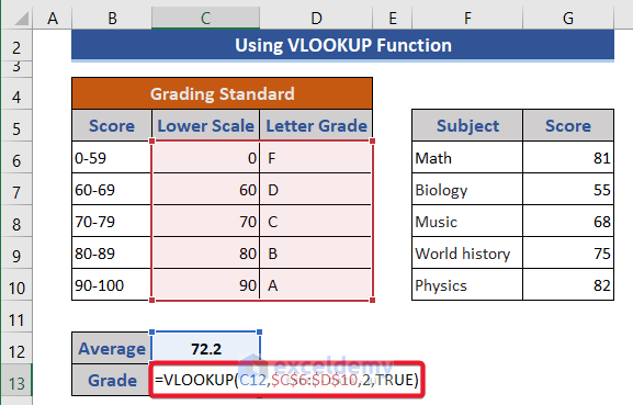
Method 3 – Use the VLOOKUP Function to Get the Average Letter Grades
Steps:
- Add a new column to the dataset. This column contains the lowest score of each level.
- Enter the VLOOKUP formula in C13.
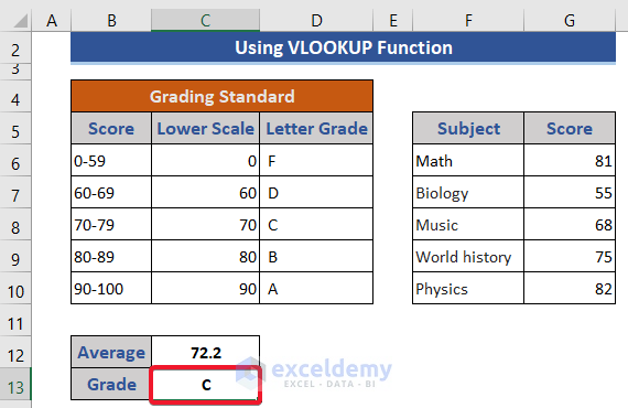
=VLOOKUP(C12,$C$6:$D$10,2,TRUE)
- Press Enter.
Method 4 – Combine the MATCH & INDEX Functions
The MATCH function returns the relative position of an item in an array that matches a specified value in a specified order.
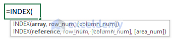
The INDEX function returns a value or reference of the cell at the intersection of the particular row and column in a given range.
Steps:
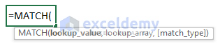
- Enter the formula in C13.
=INDEX(D6:D10,MATCH(C12,C6:C10,1))
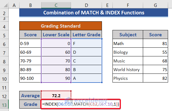
- Press Enter to see the result.

Formula Breakdown
- MATCH(C12,C6:C10,1)
finds a match for C12 in C6:C10. If it finds a value less than C12 in that range, it shows the row number.
Result: 3
- INDEX(D6:D10,MATCH(C12,C6:C10,1))
shows the value of the corresponding row in D6:D10.
Result: C
Read More: How to Calculate Average Percentage of Marks in Excel (Top 4 Methods)
Related Articles
- How to Calculate Percentage of Marks in Excel (5 Simple Ways)
- Excel Formula for Pass or Fail with Color (5 Suitable Examples)
- How to Apply Percentage Formula in Excel for Marksheet (7 Applications)
- How to Calculate Grade Percentage in Excel (3 Easy Ways)

