Download the Practice Workbook
4 Simple Steps to Calculate a Grade Using the IF Function in Excel
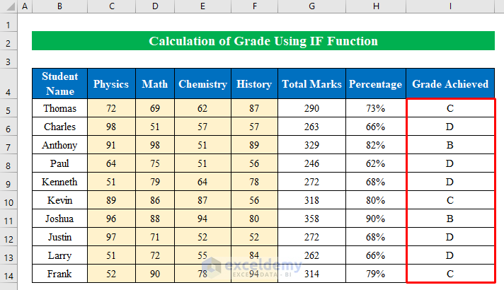
Step 1 – Create a Dataset with Appropriate Information
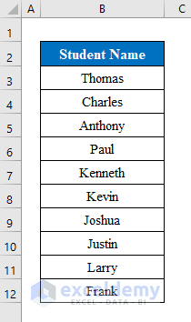
- Suppose we have a list of Student Names in our workbook.
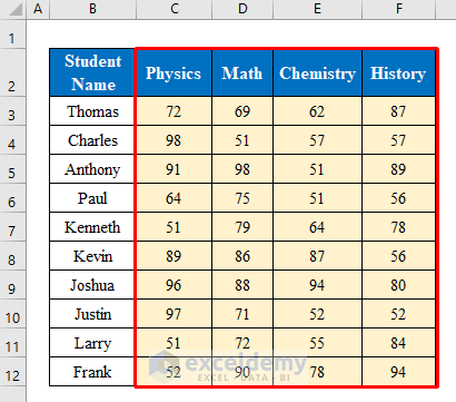
- Add the scores in different subjects for those students.
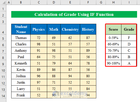
- Add the condition of the grades.
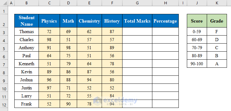
- We will add 3 columns where we will calculate the Total Marks, Percentage, and Grade Achieved.
 Read More: How to Make a Grade Calculator in Excel (2 Suitable Ways)
Step 2 – Calculate the Total Marks
- Choose cell G5 and apply the following formula-
=SUM(C5:F5)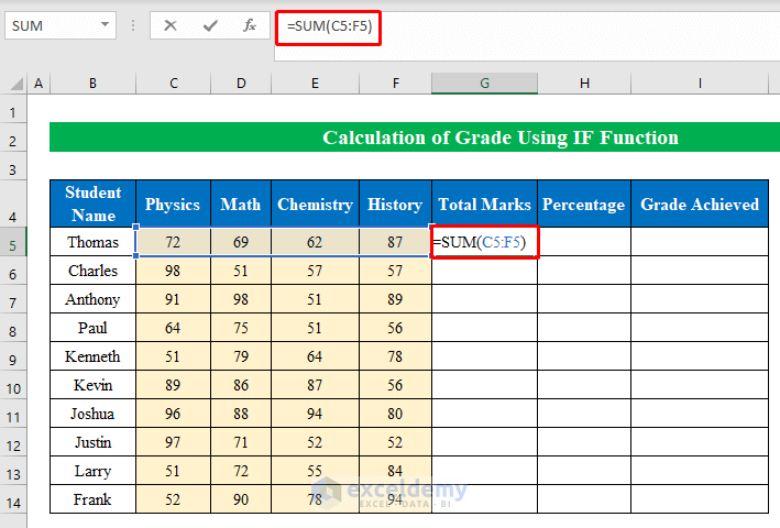
- Press Enter to get the output.
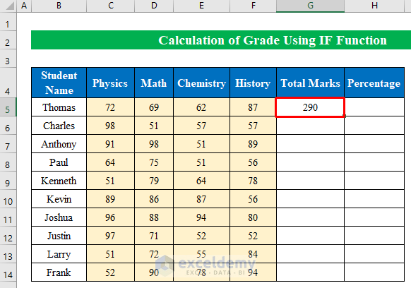
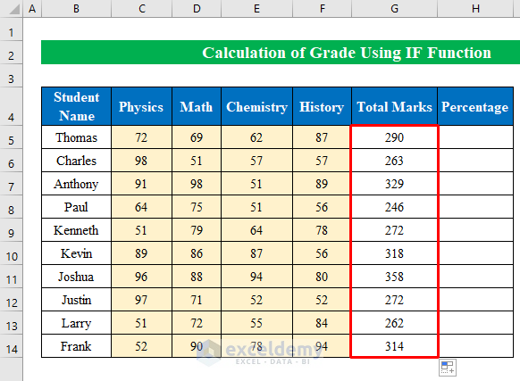
- Drag the fill handle down to fill all the cells.
Read More: How to Calculate Letter Grades in Excel (6 Simple Ways)
Similar Readings
- Excel Formula for Pass or Fail with Color (5 Suitable Examples)
- Calculate Average Percentage of Marks in Excel (Top 4 Methods)
- How to Calculate Grade Percentage in Excel (3 Easy Ways)
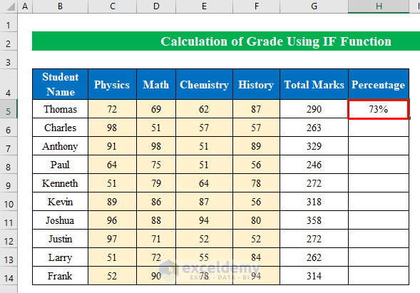
Step 3 – Calculate a Percentage from Total Marks
- Select cell H5.
- Insert the following.
=G5/400We divided by 400 because we have four subjects with 100 max score each.
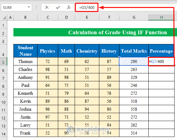
- Hit the Enter button to continue.
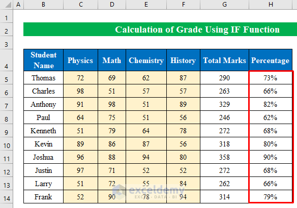
- Drag the fill handle down to get the percentage scored by all students.
Read More: How to Calculate Percentage of Marks in Excel (5 Simple Ways)
Step 4 – Apply the IF Function to Calculate the Grade
- Choose cell I5
- Put the following formula in the chosen cell:
=IF(H5>=90%,"A",IF(H5>=80%,"B",IF(H5>=70%,"C",IF(H5>=60%,"D","F"))))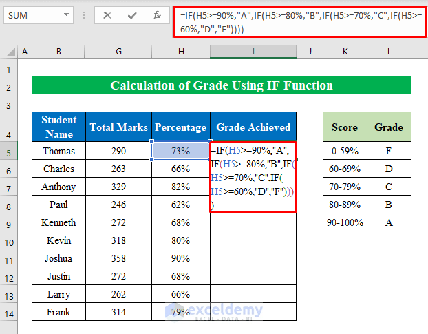
- Press Enter and pull the fill handle down to fill the cells with the given condition.
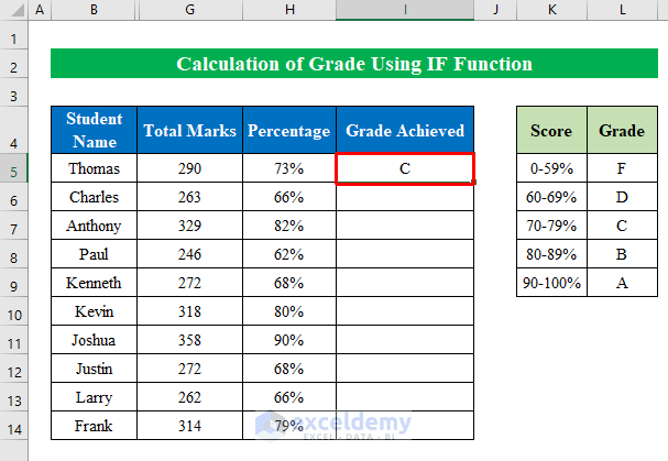
- We have successfully calculated grades using the IF function in excel.
Read More: How to Apply Percentage Formula in Excel for Marksheet (7 Applications)
Related Articles
- How to Calculate Subject Wise Pass or Fail with Formula in Excel
- Make Result Sheet in Excel (with Easy Steps)
- How to Make Automatic Marksheet in Excel (with Easy Steps)
- Calculate Grades with Weighted Percentages in Excel


thank so much I enjoy your teaching approach even a novices will understand it, just that I could not access paid course due to word press troubleshooting issue
Hello Ayokanmi,
Thanks for your appreciation. You are most welcome. Our paid courses are in Udemy not in WordPress. But we have 7500++ free tutorials and 340+ YouTube videos. You can explore these learning materials for free.
Regards
ExcelDemy
wow, It did not work at all. just keep getting error messages. even copy and pasted.
Hello Bob,
Thank you for your feedback! I’m sorry to hear you’re encountering errors. To assist you better, could you please share the specific error message you’re receiving? Also, double-check that your cell references and formula syntax match the example provided.
Sometimes, small differences like extra spaces or missing parentheses can cause issues. I’d be happy to guide you through it!
Regards
ExcelDemy
every thing is possible
Hello Felix Kiptoo,
Absolutely! With the right formulas and logic, Excel can handle almost anything. Let us know if you have any questions!
We are here to help you.
Regards
ExcelDemy
thing change
Hello Felix Kiptoo,
Yes, things do change! Excel functions keep evolving, making tasks even easier. Let us know if you need any help with the IF function!
Regards
ExcelDemy