How to Make Automatic Marksheet in Excel (with Easy Steps)

Sheet1 contains the personal details, numbers, and grading of each student.

Sheet2 contains the mark sheet template. We inserted a bold outside border.

Step 1 – Insert Personal Details

Insert a roll number in Cell E8. We inserted 1.
Insert the following formula in Cell E9 to get the corresponding student name:

=VLOOKUP(E8,Sheet1!B2:L10,2)

Hit the Enter button for the output.

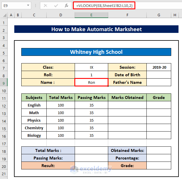
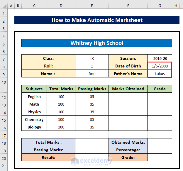
How to Make Automatic Marksheet in Excel

Apply a similar formula using the VLOOKUP function again in Cell G8 and G9 to return the date of birth and father’s name.

How to Make Automatic Marksheet in Excel

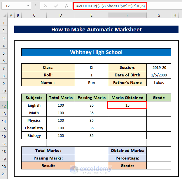
Step 2 – Insert the Obtained Marks

In Cell F12, use the following formula to get the obtained marks in English:

=VLOOKUP($E$8,Sheet1!$B$2:$L$10,6)

Hit Enter.

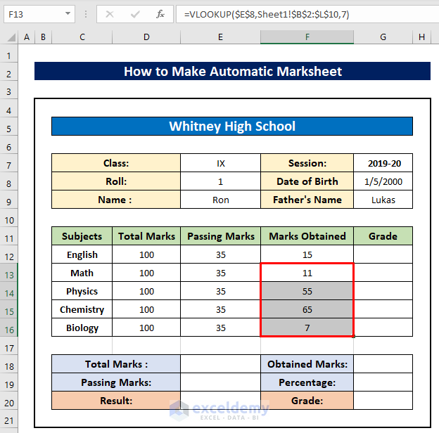
How to Make Automatic Marksheet in Excel

Repeat and modify the VLOOKUP formula to get the numbers in the other subjects. Change the column index number according to the subject name in the array of Sheet1.

Step 3 – Apply Conditional Formatting

Select the cells and go to Conditional Formatting, choose Highlight Cells Rules, then select Less Than.

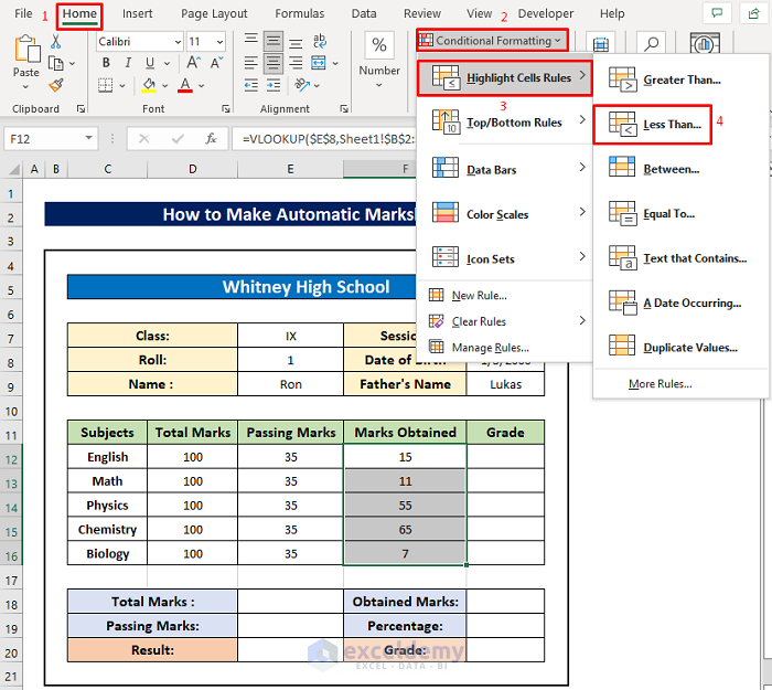
How to Make Automatic Marksheet in Excel

Insert the minimum passing number in the first box and select your desired highlight color from the second dropdown box.
Press OK.

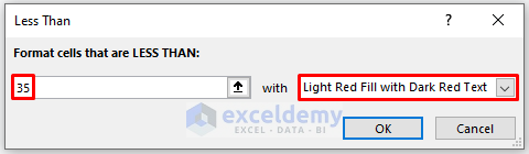
How to Make Automatic Marksheet in Excel

The numbers are highlighted with our selected color.

Step 4 – Insert Grades

Apply the following formula in Cell G12:

=IF(F12>80,"A",IF(F12>60,"B",IF(F12>50,"C",IF(F12>35,"D","F"))))

Hit the Enter button.

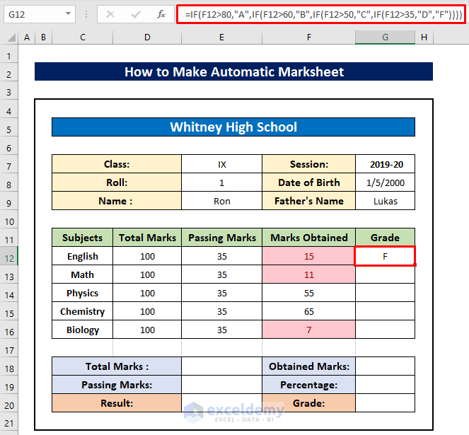
How to Make Automatic Marksheet in Excel

Use the Fill Handle tool to copy the formula for the other cells.

You will get all the grades for roll number 1.

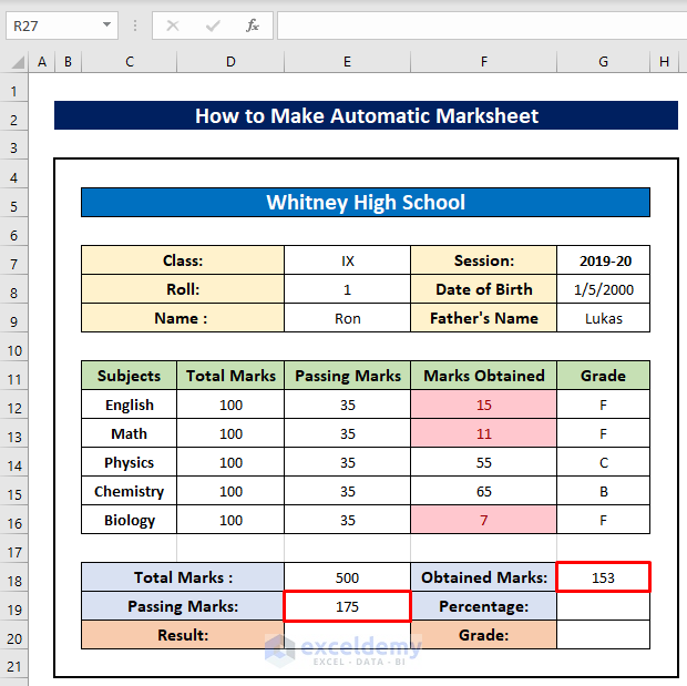
Step 5 – Calculate the Total Marks

Insert the following formula in Cell E18–

=SUM(D12:D16)

Hit Enter.

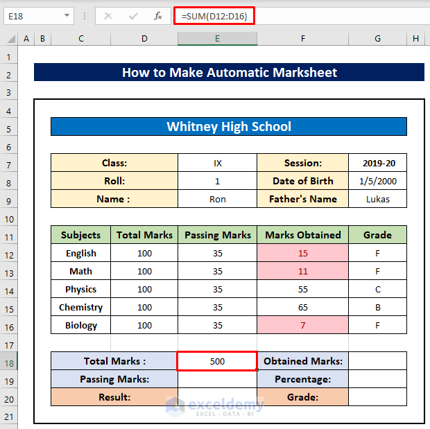
How to Make Automatic Marksheet in Excel

Find out the total passing marks and total obtained marks using the SUM formula.

How to Make Automatic Marksheet in Excel

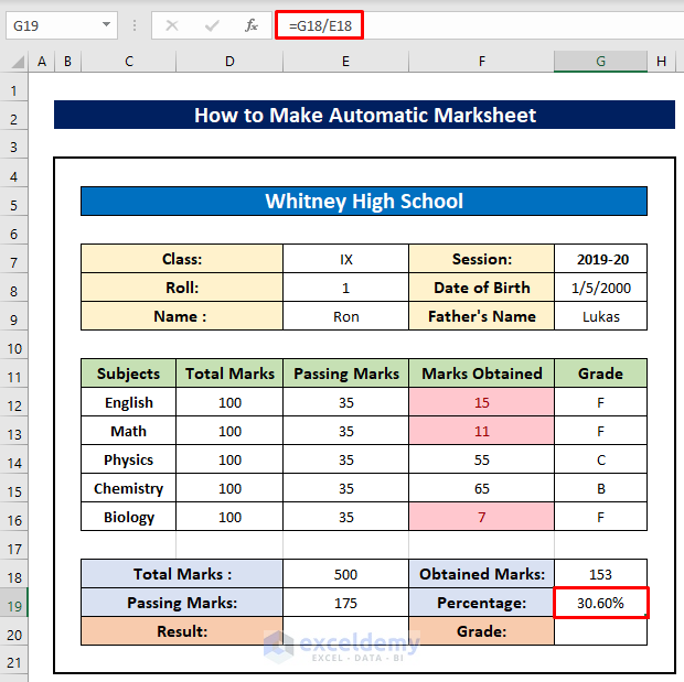
Step 6 – Calculate the Result

Insert the following formula in Cell G19:

=G18/E18

Hit Enter.

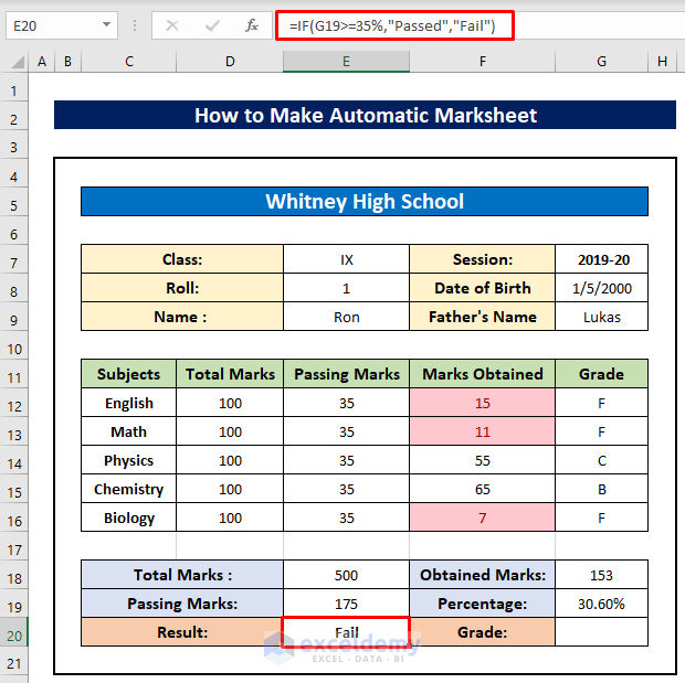
How to Make Automatic Marksheet in Excel

To determine if the student passed or failed, apply the following formula in E20.

=IF(G19>=35%,"Passed","Fail")

Press the Enter button.

How to Make Automatic Marksheet in Excel

To calculate the grade, use the following formula in Cell G20:

=IF(G19>80%,"A",IF(G19>60%,"B",IF(G19>50%,"C",IF(G19>35%,"D","F"))))

Hit Enter.

If we insert any roll number, the sheet will show the corresponding detailed result of the student.

Download the Practice Workbook

Automatic Marksheet.xlsx

Get FREE Advanced Excel Exercises with Solutions!

Sub Generate_Marksheet() Dim roll_number As String Dim name As String Dim marks As Integer Dim i As Integer i = 2 'Starting at row 2 of the Marksheets sheet Do While Worksheets("Marksheets").Cells(i, 1) <> "" 'Loop until the Roll Number column is empty roll_number = Worksheets("Marksheets").Cells(i, 1).Value name = Worksheets("Marksheets").Cells(i, 2).Value marks = Worksheets("Marksheets").Cells(i, 3).Value 'Creating a new sheet for each Roll Number Worksheets.Add(After:=Worksheets(Worksheets.Count)).name = roll_number 'Adding the Name and Marks to the sheet Worksheets(roll_number).Range("A1").Value = "Name" Worksheets(roll_number).Range("B1").Value = "Marks" Worksheets(roll_number).Range("A2").Value = name Worksheets(roll_number).Range("B2").Value = marks i = i + 1 'Moving to the next row Loop End Sub

6 Comments

Siddharth Pande Apr 1, 2023 at 6:49 PM

How to make marksheets for all roll numbers at at a click of a button in excel
- Reply
  Bishawajit Chakraborty Apr 3, 2023 at 12:16 PM
  Thank you, SIDDHARTH, for your wonderful question.
  
  Here is the solution to your question. Please take a look at the below steps.
  - Create a table with columns for Roll Number, Name, and Marks in Excel.
  - Enter the Roll Number, Name, and Marks for each student in the table.
  - Create a new sheet in Excel and name it “Marksheets”.
  - In cell A1 of the “Marksheets” sheet, enter the text “Roll Number”.
  - In cell B1, enter the text “Name”.
  - In cell C1, enter the text “Marks”.
  - Select cell A2 on the “Marksheets” sheet.
  - Go to the “Data” tab in the Excel ribbon and click on “Data Validation”.
  - In the “Data Validation” window, select “List” as the validation criteria.
  - In the “Source” field, enter the range of Roll Numbers from the table you created earlier.
  - Click “OK” to close the “Data Validation” window.
  - Repeat steps for cells B2 and C2, but select the range of Names and Marks respectively.
  - Now, select the Roll Number, Name, and Marks here.
  Here is our VBA code. Therefore, you can apply this code to solve your problem.
```
Sub Generate_Marksheet()
Dim roll_number As String
Dim name As String
Dim marks As Integer
Dim i As Integer
i = 2 'Starting at row 2 of the Marksheets sheet
Do While Worksheets("Marksheets").Cells(i, 1) <> "" 'Loop until the Roll Number column is empty
roll_number = Worksheets("Marksheets").Cells(i, 1).Value
name = Worksheets("Marksheets").Cells(i, 2).Value
marks = Worksheets("Marksheets").Cells(i, 3).Value
'Creating a new sheet for each Roll Number
Worksheets.Add(After:=Worksheets(Worksheets.Count)).name = roll_number
'Adding the Name and Marks to the sheet
Worksheets(roll_number).Range("A1").Value = "Name"
Worksheets(roll_number).Range("B1").Value = "Marks"
Worksheets(roll_number).Range("A2").Value = name
Worksheets(roll_number).Range("B2").Value = marks
i = i + 1 'Moving to the next row
Loop
End Sub
```
  Here, you will see the final result in another sheet with names and marks.
  
  I hope this may solve your issue.
  
  Bishawajit, on behalf of ExcelDemy
Idrissa A.Kamara Jul 15, 2024 at 6:54 PM

thanks very much for providing the relevant materials and tutorial, it has helped me improve my intelligency and skill in excell.
God bless
- Reply
  Shamima Sultana Jul 16, 2024 at 12:19 PM
  
  Hello Idrissa A.Kamara,
  
  You’re most welcome! I’m glad to hear that the materials and tutorial have been helpful in enhancing your Excel skills and intelligence. Your dedication to learning and improvement is truly inspiring. God bless you as well, and if you ever need further assistance or have more questions, feel free to reach out. Keep up the great work!
  Keep leaning Excel with ExcelDemy.
  
  Regards
  ExcelDemy
Nithin Aug 7, 2024 at 9:22 AM

My project for the Deep Learning is
Firstly there will be question paper and answer sheet, Firstly we have to scan question paper and It should recognise the question number and marks for that question and then we have to scan the answer sheet it should map the question and recognise the marks given and these all should be directly made as an excel file.
Give the process on how to do the project. Once can u please explain how to do it.
- Reply
  Shamima Sultana Aug 7, 2024 at 2:09 PM
  
  Hello Nithin,
  
  Your deep learning projects some of the tasks you can accomplish in Excel, such as organizing data and performing calculations. But the full scope of your project would require additional software and programming.
  
  1. You will need to use Optical Character Recognition(OCR) software to scan the question paper and answer sheet.
  It will recognize and extract question numbers and their corresponding marks.
  
  2. Then use Python scripts to process OCR output, map questions to answers, and recognize marks.
  
  3. Finally you can use Python libraries like pandas and openpyxl to create and format an Excel file with the extracted data.
  
  Regards
  ExcelDemy

How to Make Automatic Marksheet in Excel (with Easy Steps)

Step 1 – Insert Personal Details

Step 2 – Insert the Obtained Marks

Step 3 – Apply Conditional Formatting

Step 4 – Insert Grades

Step 5 – Calculate the Total Marks

Step 6 – Calculate the Result

Related Articles

Leave a reply Cancel reply