Download Practice Workbook
6 Easy Steps to Make Result Sheet in Excel
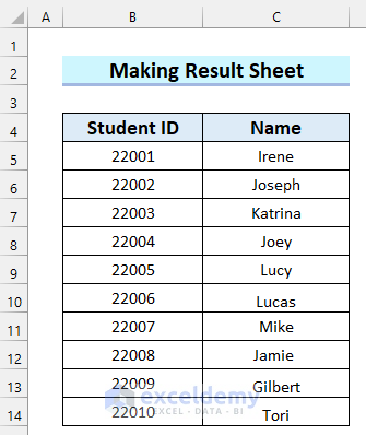
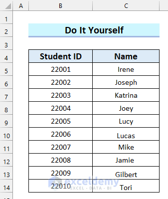
We have taken the following dataset, which contains the Student ID and Name. We’ll make a result sheet for these students.
Step 1 – Entering Data
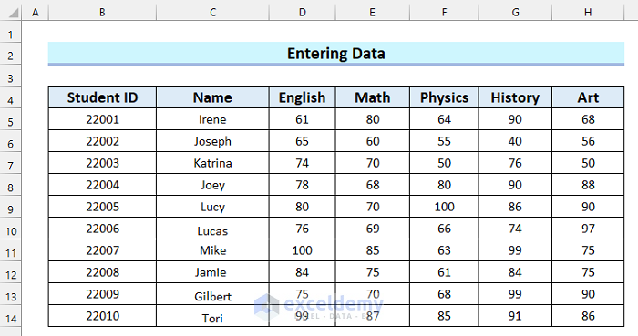
- Make columns for the subjects you have. We made columns for English, Math, Physics, History, and Art.
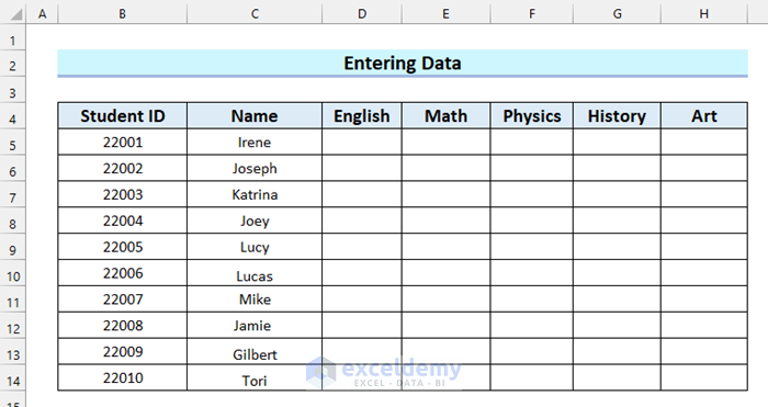
- Insert the obtained marks for these subjects for each student.
Read More: How to Make Automatic Marksheet in Excel (with Easy Steps)
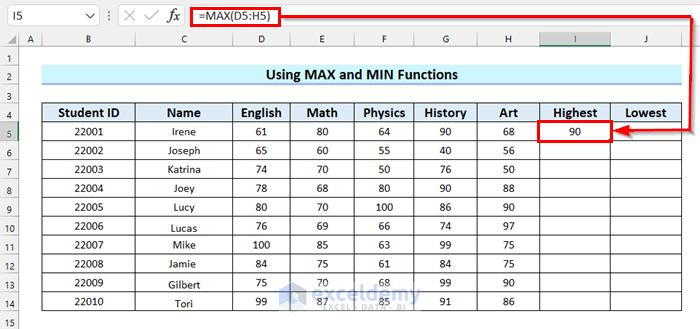
Step 2 – Using MAX and MIN Functions to get Highest and Lowest Scores
- Select the cell where you want the Highest marks. We selected cell I5.
- Insert the following formula.
=MAX(D5:H5)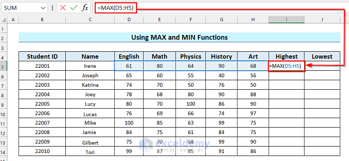
- Hit Enter.
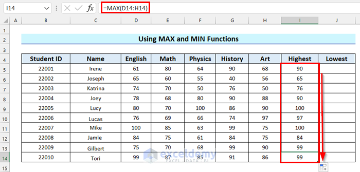
- Drag the Fill Handle to copy the formula.
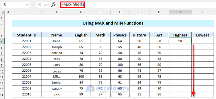
- Here’s our result.
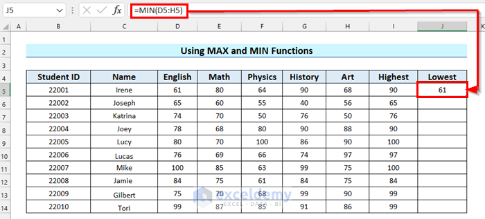
- Select the cell where you want the Lowest number. We selected cell J5.
- Insert the following formula.
=MIN(D5:H5)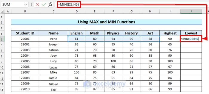
- Press Enter to get the result.
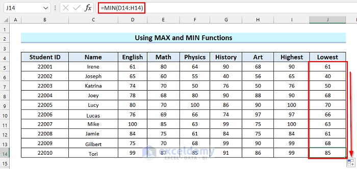
- Drag the Fill Handle down to copy the formula.
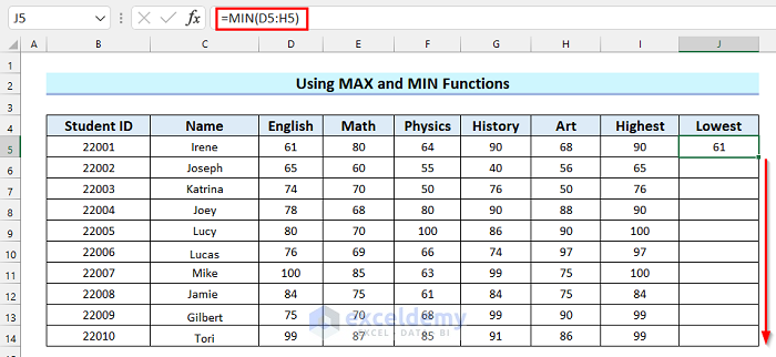
- Here’s our result.
Read More: How to Calculate Percentage of Marks in Excel (5 Simple Ways)
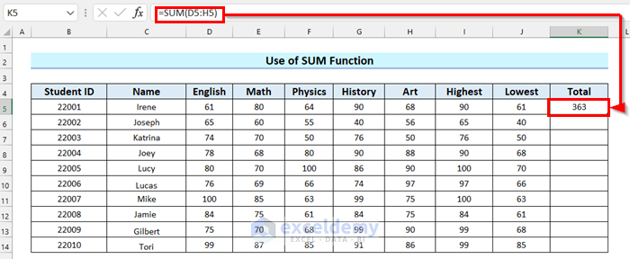
Step 3 – Use the SUM Function to Get the Total Obtained Marks for Each Student
- Select the cell where you want to calculate the Total marks. We selected cell K5.
- Insert the following formula.
=SUM(D5:H5) 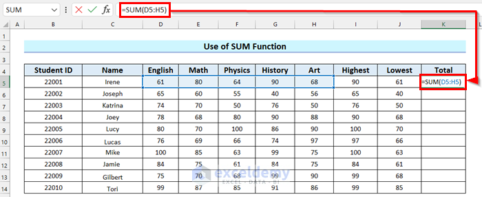
- Hit Enter.
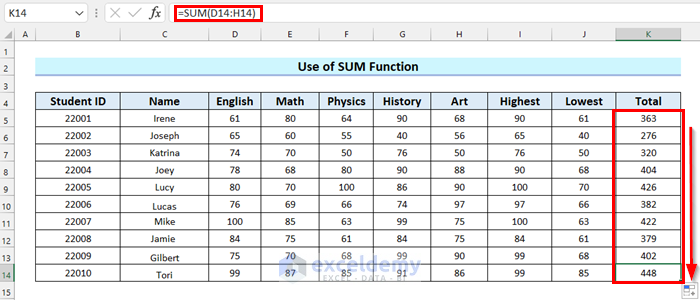
- Drag the Fill Handle down to copy the formula.
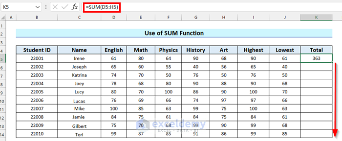
- Here’s our result.
Read More: How to Apply Percentage Formula in Excel for Marksheet (7 Applications)
Similar Readings
- How to Calculate Letter Grades in Excel (6 Simple Ways)
- How to Calculate Grade Percentage in Excel (3 Easy Ways)
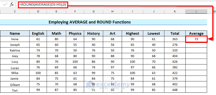
Step 4 – Using AVERAGE and ROUND Functions in the Result Sheet
- Select the cell where you want your Average marks.
- Insert the following formula in the selected cell.
=ROUND(AVERAGE(D5:H5),0)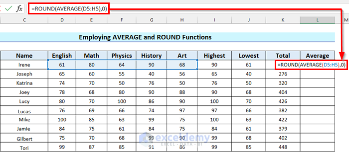
Formula Breakdown
- AVERAGE(D5:H5) —-> Here, the AVERAGE function will return the average of the cell range D5:H5.
- Output: 72.6
- ROUND(AVERAGE(D5:H5),0) —-> turns into
- ROUND(72.6,0) —-> Here, the ROUND function will return the rounded number to the given num_digits which is 0 in this case.
- Output: 73
- ROUND(72.6,0) —-> Here, the ROUND function will return the rounded number to the given num_digits which is 0 in this case.
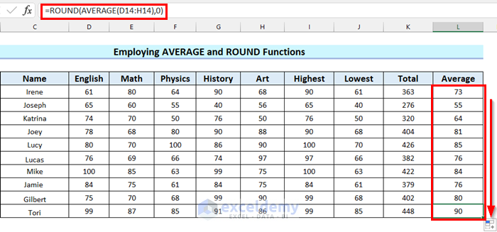
- Hit Enter.
- Drag the Fill Handle down to copy the formula.
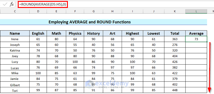
- Here’s our result.
Read More: How to Calculate Average Percentage of Marks in Excel (Top 4 Methods)
Step 5 – Using a Nested IF Function to Show Grades
We’ll use a general formula to assign grades based on the average marks.
- We hid the columns for marks for each subject since we no longer need to reference them.
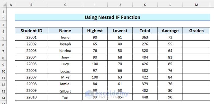
- Select the cell where you want to show your Grades. We selected cell M5.
- Insert the following formula.
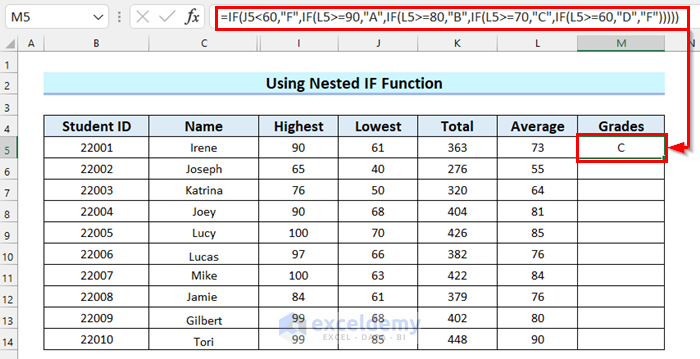
=IF(J5<60,"F",IF(L5>=90,"A",IF(L5>=80,"B",IF(L5>=70,"C",IF(L5>=60,"D","F"))))) 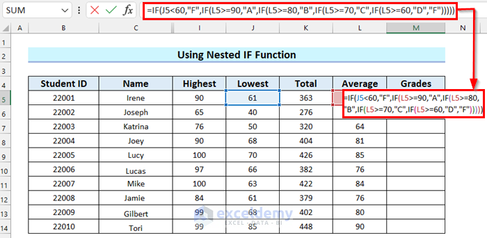
Formula Breakdown
The nested IFs will check the average score from column L against grade thresholds. The first IF checks if the student passed or failed (<60 is Fail), and each nested IF will check for a grade (90, 80, 70, 60 for A, B, C, D). If the score doesn’t fulfill the criteria for one of the grades, the if_else argument will go to the next IF.
- Hit Enter.
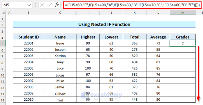
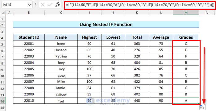
- Drag the Fill Handle down to copy the formula.
- Here’s our result.
Read More: How to Compute Grades in Excel (3 Suitable Ways)
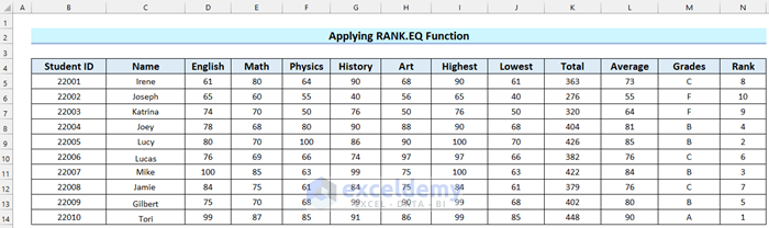
Step 6 – Applying the RANK.EQ Function in Result Sheet to Rank Students
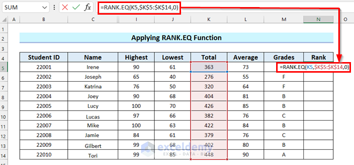
- Select the first cell where you want the Rank. We selected cell N5.
- Insert the following formula.
=RANK.EQ(K5,$K$5:$K$14,0)The second argument 0 indicates descending order, so student ranked 1 will have the highest score.
- Press Enter.
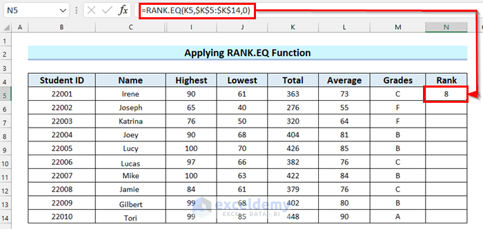
- Drag the Fill Handle to copy the formula.
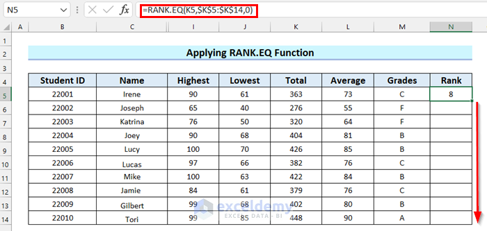
- We have copied the formula to all the cells and thus ranked the students.
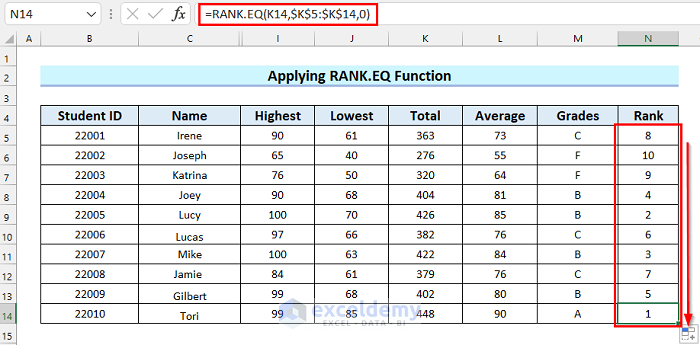
- Unhide the hidden columns so that you can see the final result sheet in Excel.
Read More: How to Make a Grade Calculator in Excel (2 Suitable Ways)
Practice Section
We have provided a simple dataset you can use to practice.


This step by step is very helpful to me. Can I have a full copy in pdf file and more practical sessions.
Thanks
Hi Robert Bakinam,
Here, you will get the full copy in pdf Marking Result Sheet.
Regards
Shamima Sultana
Project Manager | ExcelDemy
Thanks this is very useful. Please how can i go about it, if i have a report/result form in another worksheet and i want a situation when i click on any of the students name, the marks and grades in the form changes to the student’s grade
Dear Kay,
To get a customized templates you can contact with us through this Email: [email protected]
Regards
ExcelDemy
thank you very much .
Hello Naziom,
You are most welcome.
Regards
ExcelDemy
Thanks, I could learn something about xls student result sheet.
Hello Mohammad Hossain,
You are most welcome. Thanks for your appreciation an feedback. Glad to hear that our article helped you to create a student result sheet.
Keep exploring Excel with ExcelDemy!
Regards,
ExcelDemy