Download Practice Workbook
Download the practice workbook from here.
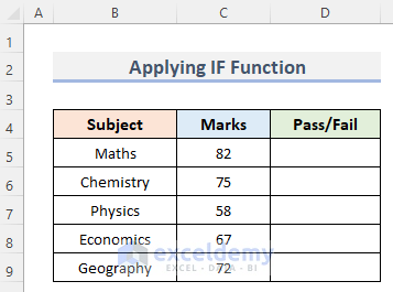
Method 1 – Apply Excel IF Function to Calculate Subject Wise Pass or Fail
Suppose we have a dataset in Excel that contains the Subjects and Marks of a student.
Steps:
- Select the cell (D5) where you want to show the result.
- Type the following formula:
=IF(C5<70, "Fail","Pass")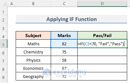
Here, C5 is the Marks of Maths. This formula checks if Marks is less than 70, resulting in Fail if true, or Pass otherwise.
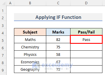
- Hit the Enter key to see the result.
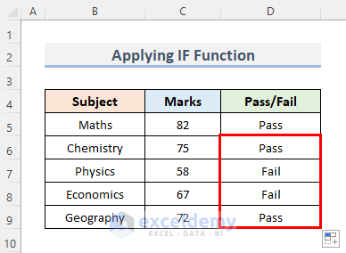
- Drag the Fill Handle to get the result of all the Subjects.
Read More: How to Make Automatic Marksheet in Excel (with Easy Steps)
Similar Readings
- How to Apply Percentage Formula in Excel for Marksheet (7 Applications)
- How to Calculate Average Percentage of Marks in Excel (Top 4 Methods)
- Calculate Grade Percentage in Excel (3 Easy Ways)
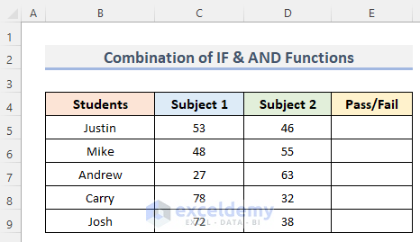
Method 2 – Get Subject Wise Pass or Fail by Combining IF & AND Functions
Consider a dataset (B4:E9) in Excel which contains the marks of two subjects of some Students. A student passes if both scores are above 35.
Steps:
- Select the desired cell (E5) to place the result.
- Copy this formula:
=IF(AND(C5>=35,D5>=35),"Pass","Fail")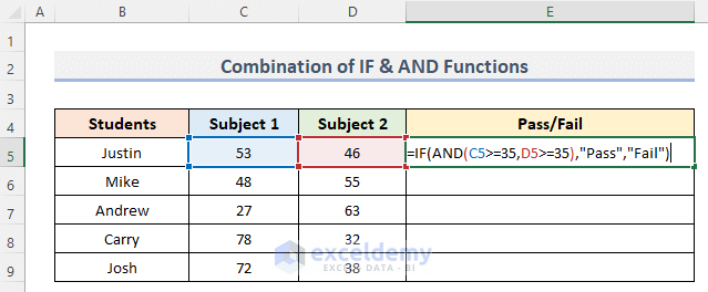
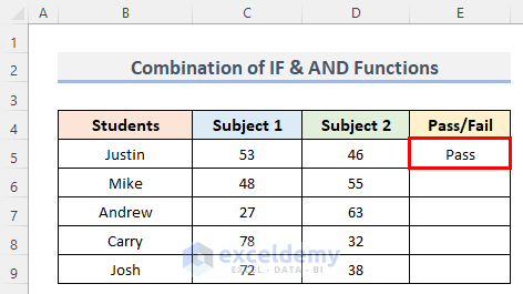
- Press Enter and see the result of the first student.
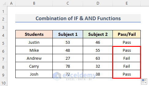
- After dragging the Fill Handle, we can see the result of the rest of the Students.
Read More: How to Make a Grade Calculator in Excel (2 Suitable Ways)
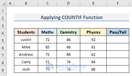
3. Use Formula with COUNTIF Function to Find Pass or Fail in Excel
Here’s a dataset (B4:F9) in Excel which contains the marks in Maths, Chemistry and Physics of some Students. If a student gets 70 or more in at least two subjects then he will Pass.
Steps:
- Select the cell F5.
- Use this formula:
=IF(COUNTIF(C5:E5,">=70")>=2,"Pass","Fail")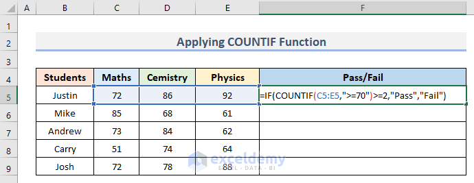
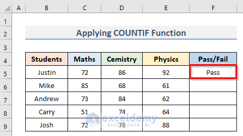
- Press the Enter button to get the result. In our case, the result is ‘Pass’ as it satisfies the requirements.
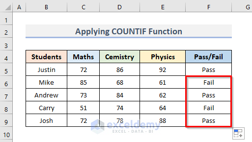
- Drag the Fill Handle to find the result of the other Students.
Read More: How to Compute Grades in Excel (3 Suitable Ways)
Related Articles
- How to Calculate Grades with Weighted Percentages in Excel
- Calculate Grade Using IF function in Excel (with Easy Steps)
- How to Calculate Letter Grades in Excel (6 Simple Ways)
- Calculate Percentage of Marks in Excel (5 Simple Ways)


Math Physcis Chemistry Biology Total Rank
Ram 86 79 75 89 329
Mohan 93 54 76 84 307
Shohan 61 Absent 55 81 197
Gita 57 74 56 86 273
Mita 60 58 67 Absent 185
Rita 94 72 62 83 311
if a student in any of the exams his/her rank column should be denote Fail otherwise his/her rank in the class. To do this use suitable formula in MS Excel
Dear KRISHNA KANT,
Thank you for giving your time to read this article. You want to know the formula to calculate the ranks and denote “Fail” if a student is absent in any of the exams. Read the following section for details.
Assuming the given data is placed in columns B to G, and the student rank will be shown in column H.
In cell H5, enter the following formula:
=IF(COUNTIF(C5:F5,"Absent")>0, "Fail",RANK(G5,$G$5:$G$10,0))Drag the formula down to apply it to the rest of the cells in column H.
The overall formula checks if there are any cells with the value “Absent” in range C5:F5. If there exists, it returns “Fail“. Otherwise, it calculates the rank of the value in G5 within the range G5:G10 in ascending order.
The student’s total score and rank are displayed in column G, and column H respectively. If a student is “Absent” in any of the exams, their rank will be denoted as “Fail.”
If you have any more queries, please let us know in the comments.
Regards
Annyca Tabassum
Team ExcelDemy
How to write the formula if the student passes all 3 subjects and it will show pass, if the student passes at least 1 subject it will show Try again and if the student fails all three subjects it will show fail?
Dear CARLO MUNDAN,
I hope you are doing well and thanks for your query.
Assuming the marks of three subjects are in the range C5 to E5, the result will be shown in cell F5.
The following formula gets your desired answer.
=IF(COUNTIF(C5:E5, “>=70”)=3, “Pass”, IF(COUNTIF(C5:E5, “>=70”)>=1, “Try again”, “Fail”))
Here, I have used two COUNTIF functions along with an IF function inside an IF function to get the result you desired. Drag the formula down to apply it to the rest of the cells.
If you have any more queries, please let us know in the comments.
Regards
Team ExcelDemy
suppose there are 5 subjects and Raju failed in one subject then how to use formula even Percentage is 60 percent bcz Raju has got more numbers in remaining subjects?
Hello Abdul
Thanks for reaching out and posting your comment. You want to highlight the scenario where a student, Raju, fails in one subject out of five but still manages to achieve a high percentage overall due to scoring well in the remaining subjects.
Basically, you want to ensure that Raju isn’t labelled a failure just because he fails one subject. In your view, Raju’s overall performance across all subjects should involve when determining his pass/fail status, not just the grade in one subject.
Hopefully, you have found the idea helpful. Good luck.
Regards
Lutfor Rahman Shimanto
ExcelDemy