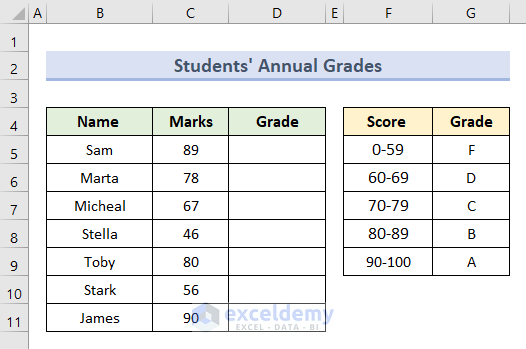
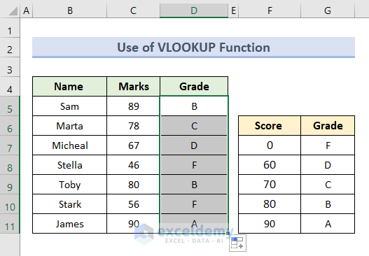
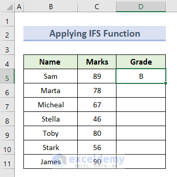
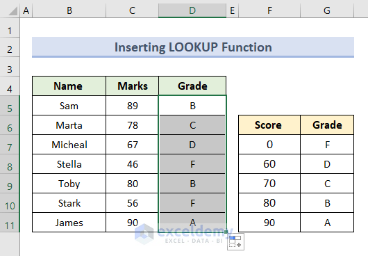
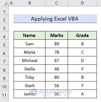
How to Calculate Letter Grades in Excel (6 Simple Ways)

The result in our transcripts is represented by the letter grades at the end of any exam. But it becomes difficult for the teachers to calculate grades one by one for each student. Therefore, excel has offered certain formulas to calculate letter grades. In this article, we will learn how to calculate letter grades in Excel in 6 simple ways.

Here is an annual grade sheet of 7 students in an institution with names and marks. Along with that, we also have grades based on the range of scores.

Now, we will calculate the letter grades of the students.

1. Using the VLOOKUP Function to Calculate Letter Grades in Excel

In this first one, we will use the VLOOKUP function to get letter grades in Excel. Let’s go through the process below:

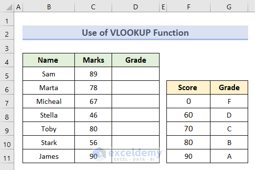
First, change the Score from range to single numbers as VLOOKUP calculates defining the series of numbers as a table array automatically.

Next, insert this formula in cell D5.

=VLOOKUP(C5,$F$7:$G$11,2,TRUE)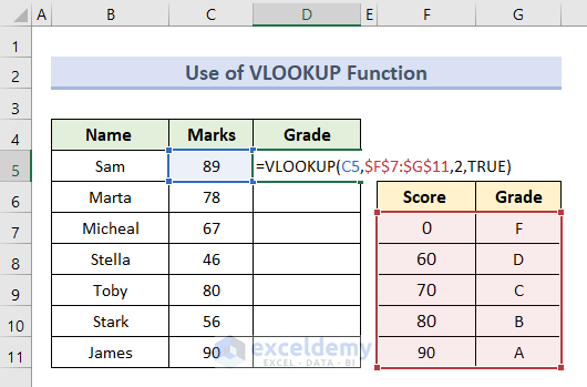

Here, C5 defines the student score that we want to calculate for the letter grade. Cell range F7:G11 is the table which the lookup value will be returned from. 2 is the column number in the lookup table to return the matched value. Lastly, TRUE is for an approximate match.

Then, press Enter.
That’s it, you can see the letter grade for the required mark.

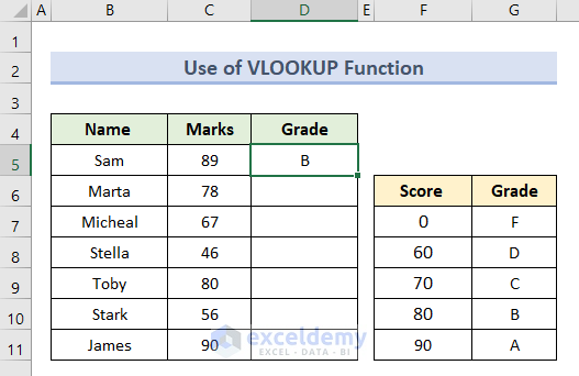
Following, use the AutoFill tool to apply the same formula for all marks.

2. Calculating Letter Grades with IF Function

At this stage, we will calculate the letter grades with the IF function in excel. Following is the step-by-step guideline:

First, insert this formula in cell D5.

=IF(C5>=90,"A",IF(C5>=80,"B",IF(C5>=70,"C",IF(C5>=60,"D","F"))))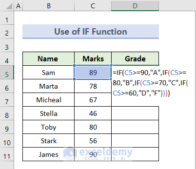

Here, the IF function is applied to return one value based on the condition given for the selected cell defining whether it is true or false. Therefore, if the student gets more than 90 the letter grade will be A, and chronologically marks less than 60 will get F.

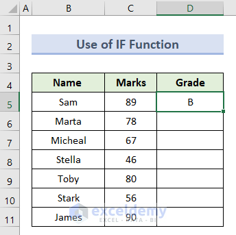
Now, press Enter.
Finally, you can see the letter grade is visible beside the marks.

Apply similar formula or drag the bottom corner of cell D5 to get the output for all the marks.

3. Apply IFS Function in Excel to Calculate Letter Grades

The IFS function also helps to calculate the letter grades in Excel. Let’s see how it works.

In the beginning, insert this formula in cell D5.

=IFS(C5>=90,"A",C5>=80,"B",C5>=70,"C",C5>=60,"D",C5<60,"F")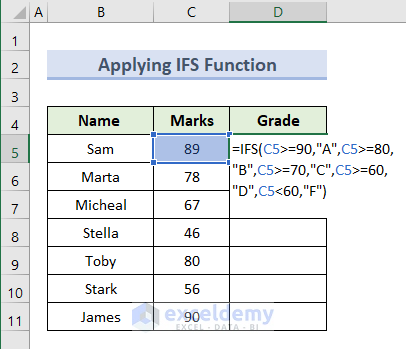

Here, the IFS function checks the successful completion of one or more conditions. After that, it returns a value that corresponds to the first TRUE condition. The conditions are based on the source dataset.

Then, press Enter.
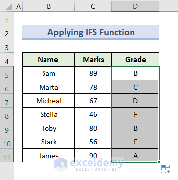
Now, you will see the letter grade based on the mark.

Follow the similar process and calculate the letter grades of other students as well.

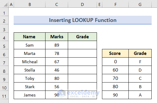
4. Insert LOOKUP Function for Letter Grades Calculation

The LOOKUP function is also very helpful to find the letter grades in excel. Follow the steps below:

At first, change the range of scores to minimum numeric values of that respect range as per this image:

Now, insert this formula in cell D5.

=LOOKUP(C5,$F$7:$F$11,$G$7:$G$11)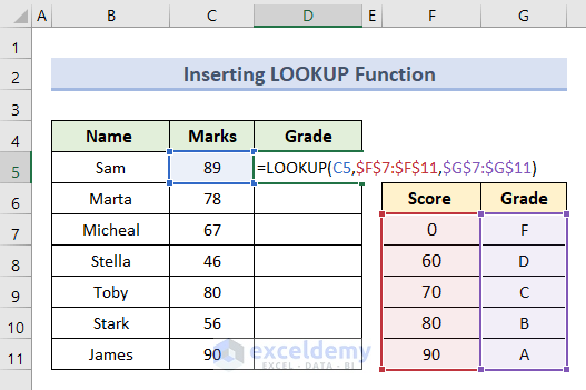

Here, C5 defines the student score that we want to calculate for the letter grade. Cell range F7:F11 is the reference which the lookup value will be returned from. Lastly, G7:G11 is the source cell range of scores.

After this, press Enter.
Lastly, use the AutoFill tool in cell range D6:D11 to get the final output.

Read More: How to Make Result Sheet in Excel

5. Finding Letter Grades Using Excel VBA Macro

Excel VBA macro is a very useful technique to calculate letter grades. Let’s check the process.

Firstly, go to the Developer tab and select Visual Basic.

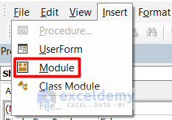
Secondly, select Module from the Insert section.

After that, insert this code on the blank page.

Sub InsertLetterGrade()

Dim i As Integer
Dim rslt As String
For i = 5 To 11
If (Cells(i, 3) >= 90) Then
   result = "A"

ElseIf (Cells(i, 3) >= 80) Then
  result = "B"

ElseIf (Cells(i, 3) >= 70) Then
   result = "C"
   
ElseIf (Cells(i, 3) >= 60) Then
   result = "D"

Else
   result = "F"
End If
Cells(i, 4).Value = result
Next i
End Sub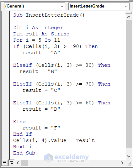

Now, click on the Run Sub button or press F5 on your keyboard.

Therefore, click on the Run in the Macros window.

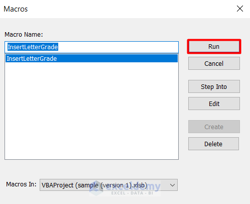
Finally, you will get all the letter grades at a time in cell range D5:D11.

6. Combining IF and AND Functions to Calculate Letter Grades in Excel

In this last method, we will find grades defining pass or fail based on the marks of each student. If one gets below 60 marks, then it will be considered a Fail. Otherwise, it’ll be considered a Pass. We will use a combination of the IF & AND functions in Excel. Let’s see how it works.

First, insert this formula in cell D5.

=IF(AND(B5,C5>=60),"Pass","Fail")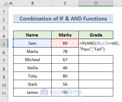

Here, the IF function is used to return one value when a condition is true. It also defines another value if it’s false for the selected cell. The AND function tests the condition if the grade is greater than or equal to 60. If all the conditions are correct, then we will get the result as TRUE. Otherwise, the result will be FALSE.

Now, press Enter.
There you will see the output.

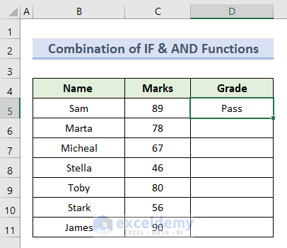
Apply the AutoFill tool to get results in cell range D6:D11.

Things to Remember

When you have a percentage instead of numbers, you will also need to define % in the logical function to get letter grades.
Make sure to lock the selected range before dragging the formula to other cells.
In the case of calculating the grades for a situation where the less number means a higher grade, then use “<” instead of “>” as the operator.

Download Practice Workbook

Get the sample file here to practice by yourself.

Calculate Letter Grades.xlsm

Conclusion

I hope it was a helpful article for you on how to calculate letter grades in Excel. Let us know your feedback in the comment box.

Get FREE Advanced Excel Exercises with Solutions!