Method 1 – Creating Reference Table to Calculate GPA
- Create a table with 3 columns and 6 rows.
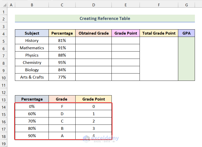
- Name the columns as Percentage, Grade, and Grade Point respectively.
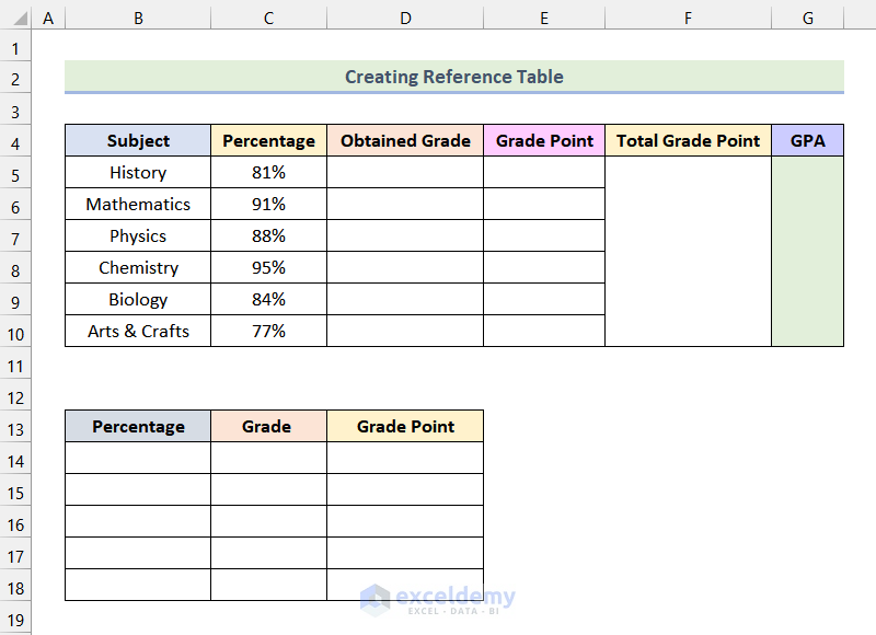
- Enter the Percentage ranges, Grades, and Grade Points as shown in the following picture.
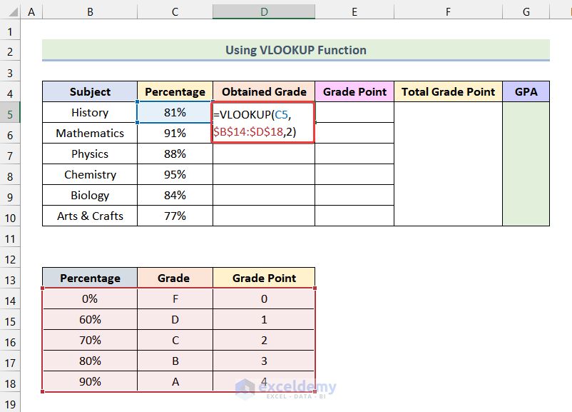
Method 2 – Using VLOOKUP Function to Calculate GPA in Excel
- Enter the following formula in cell D5.
=VLOOKUP(C5,$B$14:$D$18,2)Cell C5 refers to the obtained Percentage of History exam, the range $B$14:$D$18 represents the Reference Table that we are using to calculate GPA.
Formula Breakdown
- =VLOOKUP(C5,$B$14:$D$18,2) → It looks for a given value in the leftmost column of a given table and then returns a value in the same row from a specified column.
- C5 → lookup_value argument.
- $B$14:$D$18 → table_array argument
- 2 → col_index_num argument
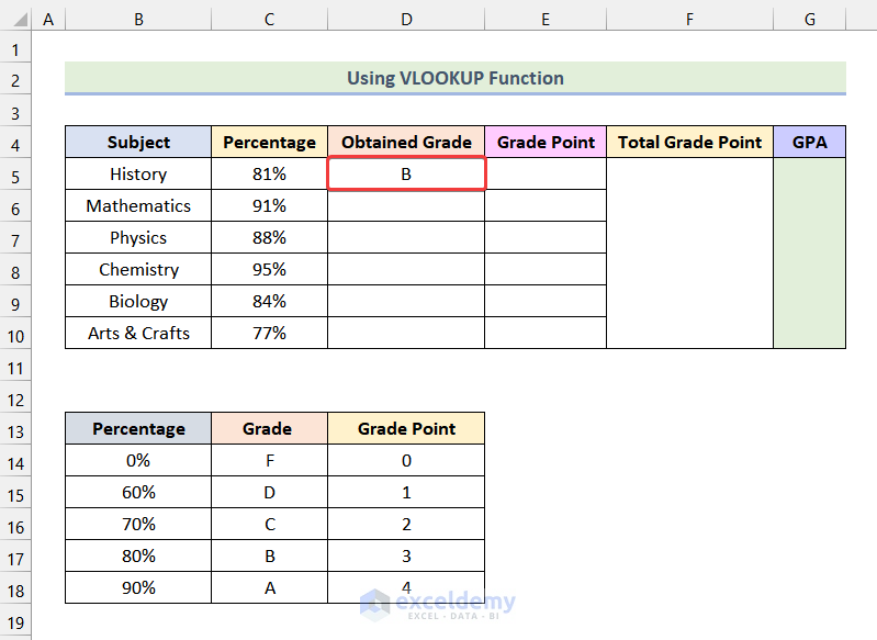
- Output → B
- Press ENTER.
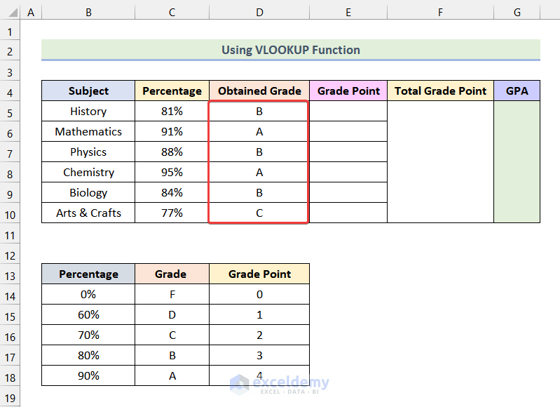
You will see the Grade of History as marked in the image given below.
- Use the AutoFill feature of Excel to get the rest of the Grades for other Subjects as shown in the following picture.
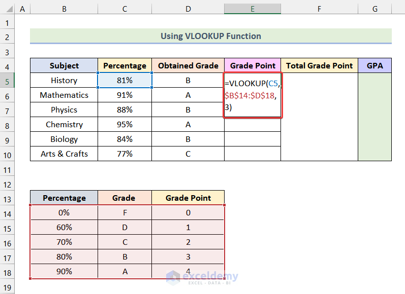
- Enter the formula given below in cell E5.
=VLOOKUP(C5,$B$14:$D$18,3)Formula Breakdown
- =VLOOKUP(C5,$B$14:$D$18,2) → It looks for a given value in the leftmost column of a given table and then returns a value in the same row from a specified column.
- C5 → lookup_value argument.
- $B$14:$D$18 → table_array argument
- 3 → col_index_num argument
- Output → 3
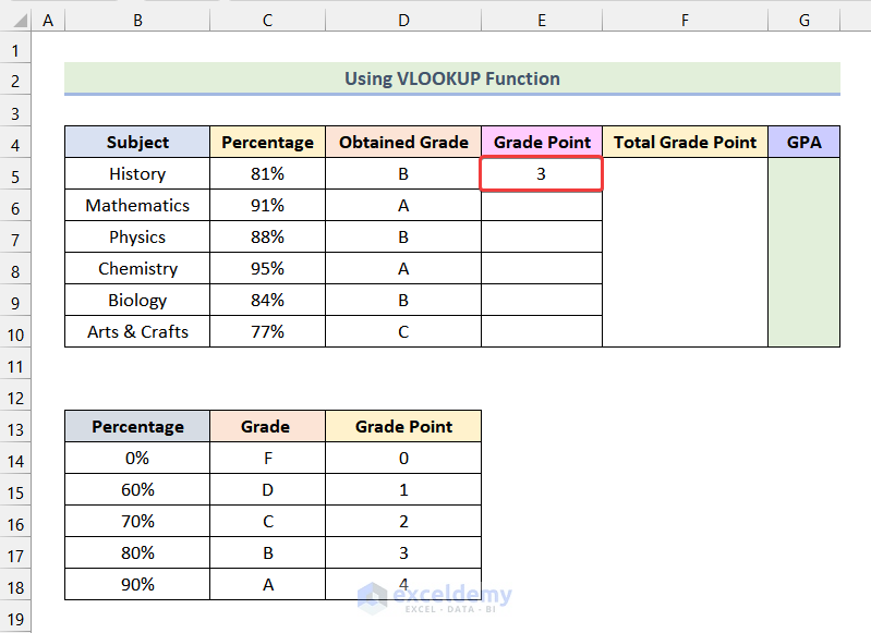
- Hit ENTER.
The Grade Point of History for Peter Rogers will be available in cell E5, as marked in the picture below.
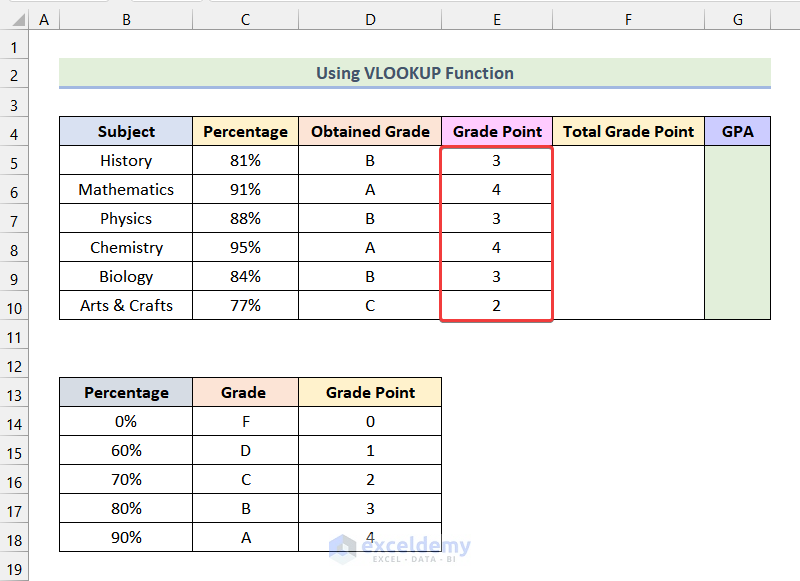
- Using the AutoFill option of Excel, you can obtain the remaining Grade Points for the rest of the Subjects.
Method 3 – Utilizing SUM and COUNTA Functions to Calculate GPA
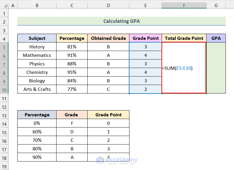
- Enter the following formula in cell F5.
=SUM(E5:E10)The range E5:E10 represents the Grade Points achieved by Peter Rogers in different Subjects.
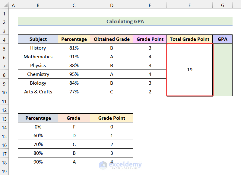
- Press ENTER.
You will see the Total Grade Point in cell F5 as marked in the following picture.
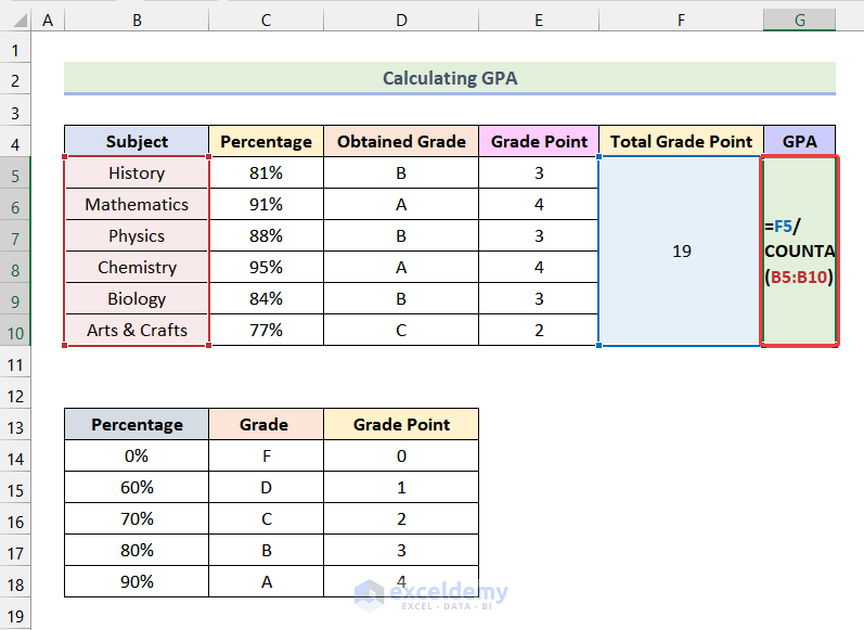
To calculate the GPA, we will use the COUNTA function.
- Enter the formula below in cell G5.
=F5/COUNTA(B5:B10)The range B5:B10 refers to the cells of the column Subject.
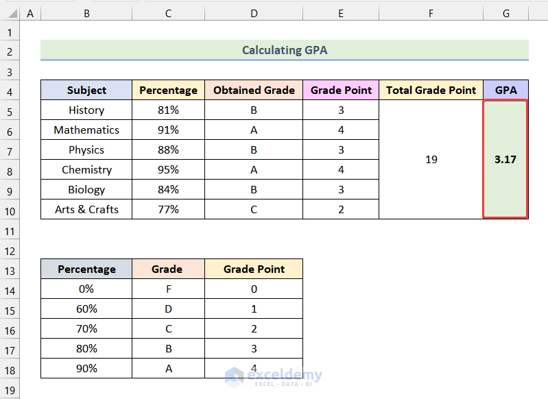
- Hit ENTER.
You will see the GPA obtained by Peter Rogers in cell G5 as demonstrated in the following picture.
Download Practice Workbook
Related Articles
- How to Average Letter Grades in Excel
- Make Result Sheet in Excel
- How to Make Automatic Marksheet in Excel
- How to Calculate Subject Wise Pass or Fail with Formula in Excel
- How to Calculate Final Grade in Excel
- How to Calculate Average Percentage of Marks in Excel
Get FREE Advanced Excel Exercises with Solutions!

