Download the Practice Workbook
5 Easy Methods to Sum Filtered Cells in Excel
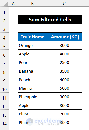
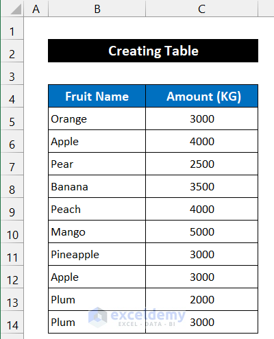
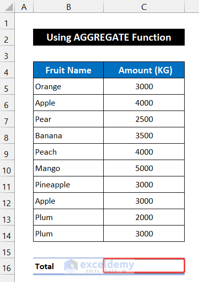
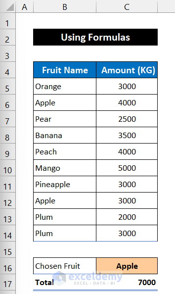
Let’s consider a dataset of some fruits and their amounts. We’ll filter the dataset for Apple and then sum up the quantity of this fruit.
Method 1 – Utilizing the SUBTOTAL Function
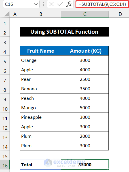
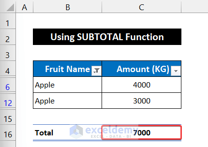
The sum of the function will be in cell C16.

Steps:
- Select cell C16.
- Insert the following formula into the cell.
=SUBTOTAL(9,C5:C14)
9 is the function number of the SUM function. The values which the function will sum are in the range of cells C5:C14.
- Press Enter.
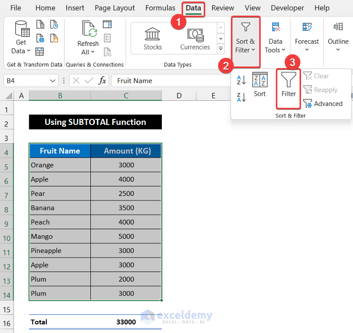
- Select the entire range of cells B4:C14.
- In the Data tab, select the Filter option from the Sort & Filter group.
- You will get two drop-down arrows in the column headers.
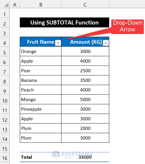
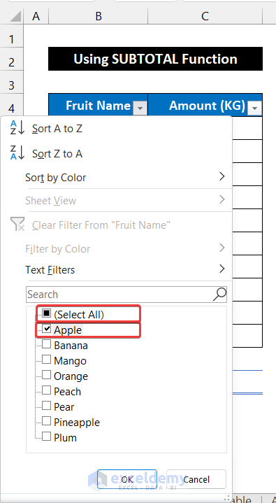
- Click the drop-down arrow of the Fruit Name column.
- Uncheck the Select All option and click on Apple only.
- Click OK.
- Here’s the result.
Read More: How to Sum Range of Cells in Row Using Excel VBA (6 Easy Methods)
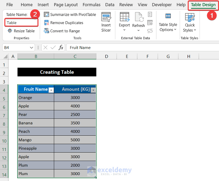
Method 2 – Sum Filtered Cells by Creating a Table in Excel
We will use the same dataset.
Steps:
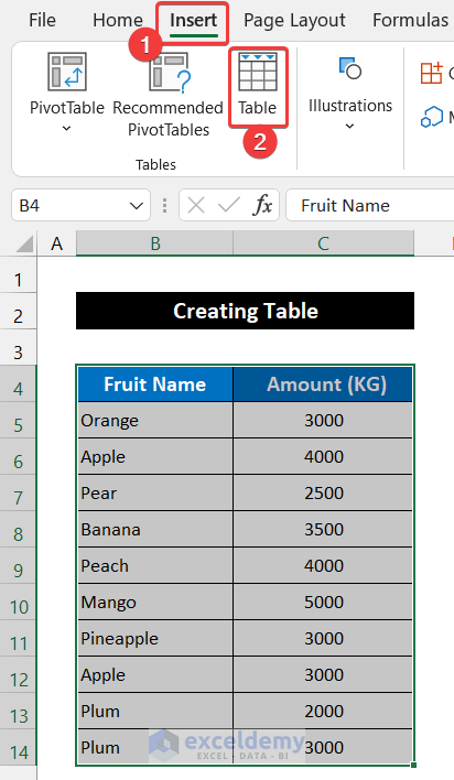
- Select the entire range of cells B4:C14.
- In the Insert tab, select Table. You can also press Ctrl + T to create the table.
- A small dialog box named Create Table will appear. Click on My table had headers and hit OK.

- The table will be created.
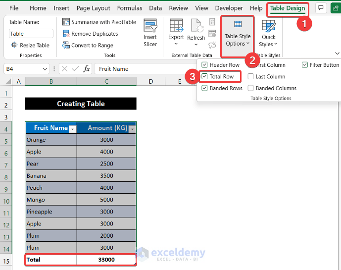
- In the Table Design tab, you can change the table name in the Properties group.
- From the Table Style Options group, click on Total Row.
- A new row will appear below the table and show the total value of column C.
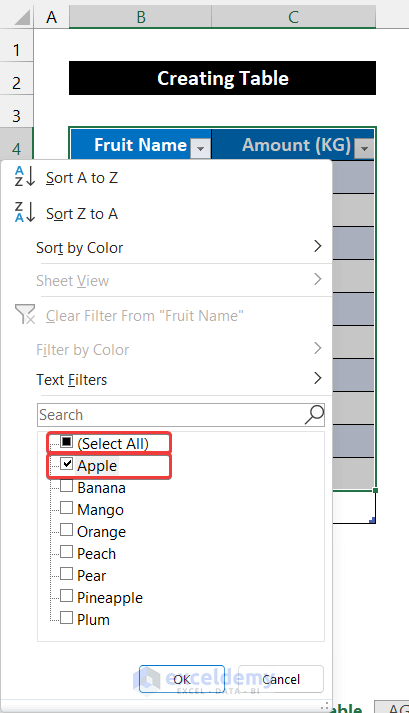
- Click on the drop-down arrow in the heading that shows Fruit Name.
- Uncheck the Select All option and select the Apple option only.
- Click the OK button to close that window.
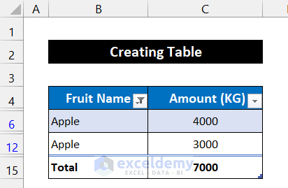
- Here’s the result.
Read More: How to Sum Selected Cells in Excel (4 Easy Methods)
Method 3 – Applying the AGGREGATE Function
We’ll use the same dataset.
Steps:
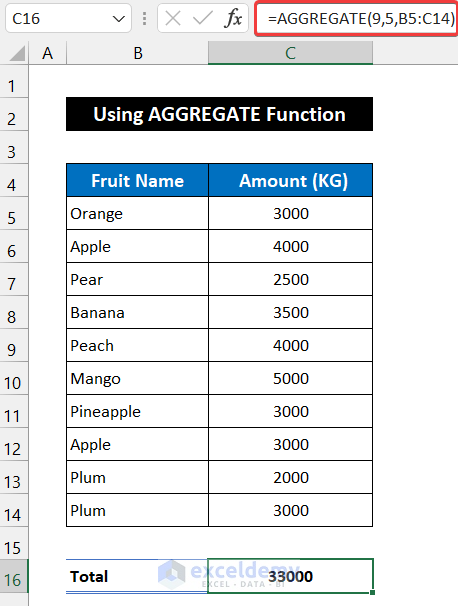
- Select cell C16.
- Use the following formula in the cell.
=AGGREGATE(9,5,B5:C14)
The first element, 9, is the function number of the SUM function. The second element, 5, makes the function ignore hidden rows. The last element is value range, C5:C14.
- Press Enter.
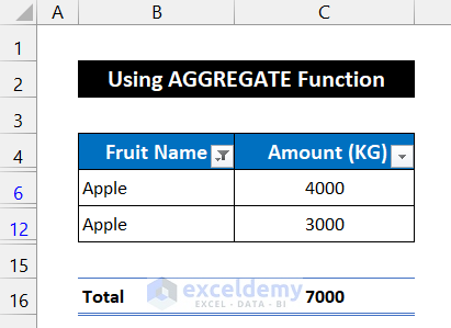
- Select the entire range of cells B4:C14.
- In the Data tab, select the Filter option from the Sort & Filter group.

- Click the drop-down in the Fruit Name column.
- Uncheck the Select All option and click on the Apple option only.

- Here’s the result.
Read More: How to Sum Only Visible Cells in Excel (4 Quick Ways)
Similar Readings
- How to Sum by Group in Excel (4 Methods)
- 3 Easy Ways to Sum Top n Values in Excel
- Sum Cells in Excel: Continuous, Random, With Criteria, etc.
- How to Sum Multiple Rows in Excel (4 Quick Ways)
Method 4 – Using a Combined Formula to Sum Filtered Cells
Steps:
- Select cell C17.
- Use the following formula in the cell.
=SUMPRODUCT(SUBTOTAL(3,OFFSET(B5:B14,ROW(B5:B14)-MIN(ROW(B5:B14)),,1)),( B5:B14=C16)*(C5:C14))
- Press Enter key on your keyboard.
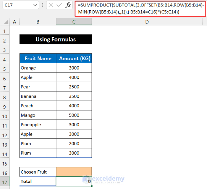
- In cell C16, write down a fruit name manually. We chose Apple to filter the sum.
- Press Enter.
- You’ll get the result.
- As an advanced method, you can insert a drop-down in C16 to select from a list of values in column C.
Breakdown of the Formula:
ROW(B5:B14): This function returns simply the row number which contains our data.
MIN(ROW(B5:B14)): This function returns the lowest row number of our dataset.
OFFSET(B5:B14,ROW(B5:B14)-MIN(ROW(B5:B14)),,1): This function returns the difference between the row number and min row number to the SUBTOTAL function.
SUBTOTAL(3,OFFSET(B5:B14,ROW(B5:B14)-MIN(ROW(B5:B14)),,1))*(B5:B14=C16)*(C5:C14): This function returns the value of quantity for Apple entities and 0 for All Other entities.
SUMPRODUCT(SUBTOTAL(3,OFFSET(B5:B14,ROW(B5:B14)-MIN(ROW(B5:B14)),,1)),( B5:B14=C16)*(C5:C14)): This function returns 7000, the sum of all Apple quantity.
Read More: [Fixed!] Excel SUM Formula Is Not Working and Returns 0 (3 Solutions)
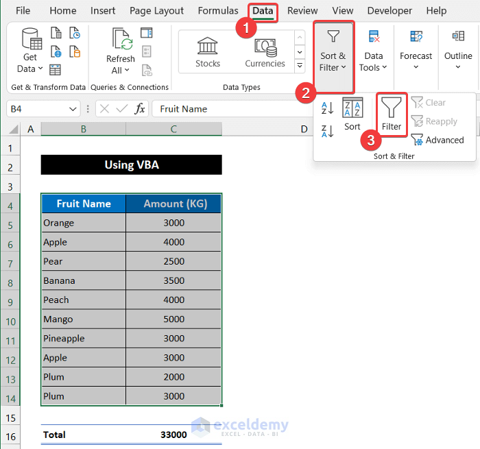
Method 5 – Embedding VBA Code
Steps:
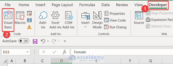
- Go to the Developer tab and click on Visual Basic. If you don’t have that, enable the Developer tab. Alternatively, press Alt + F11.
- The VBA window will appear.
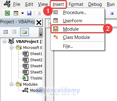
- In the Insert tab, click Module.
- Insert the following code in the empty editor box.

Function Sum_Filtered_Cells(WorkRng As Range) As Double
    Dim work_rng As Range
    Dim output As Double
    For Each work_rng In WorkRng
        If work_rng.Rows.Hidden = False And work_rng.Columns.Hidden = False Then
            output = output + work_rng.Value
        End If
    Next
    Sum_Filtered_Cells = output
End Function
- Close the Editor tab.
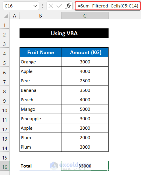
- In cell C16, use the following formula-
=Sum_Filtered_Cells(C5:C14)
- Press the Enter key.
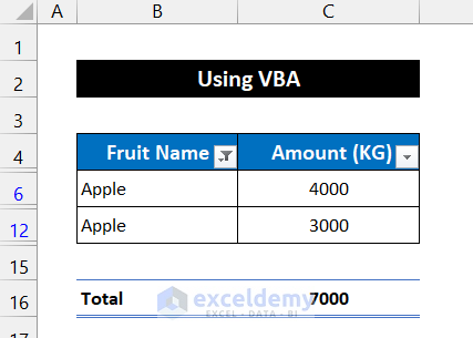
- You will get the sum of all rows in cell C16.
- Select the entire range of cell B4:C14.
- In the Data tab, select the Filter option from the Sort & Filter group.
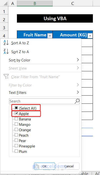
- Select the filter for Fruit Name and choose Apple.
- Here’s the result.
Related Articles
- Excel Sum If a Cell Contains Criteria (5 Examples)
- How to Vlookup and Sum Across Multiple Sheets in Excel (2 Formulas)
- Add Multiple Cells in Excel (6 Methods)
- How to Sum Rows in Excel (9 Easy Methods)
- Sum a Column in Excel (6 Methods)
- How to Sum Multiple Rows and Columns in Excel

