How to Add Multiple Cells in Excel (7 Easy Ways)

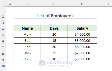
We have a list of employees of a company, their corresponding working days, and their salaries. We will use this dataset to add cells.

Method 1 – Using the AutoSum Feature to Add Multiple Cells in Excel

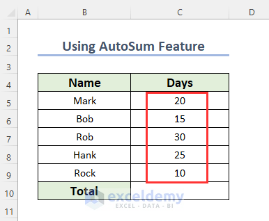
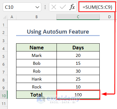
We’ll use a table of people’s names and their working days to add the working days.

Steps:

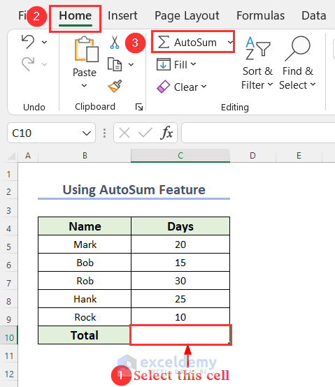
• Click on cell C10 go to the Home tab.
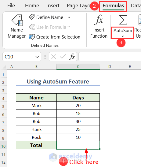
• From the Editing group of commands, click on AutoSum.

• In Cell C10, a formula appears and points to the cells we want to add.

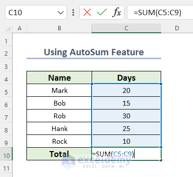
• Hit Enter.

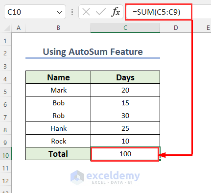
• You can also do this by going to the Formulas tab and selecting AutoSum.

The result will be the same.

Read More: How to Add Specific Cells in Excel

Method 2 – Applying an Algebraic Formula to Add Multiple Cells in Excel

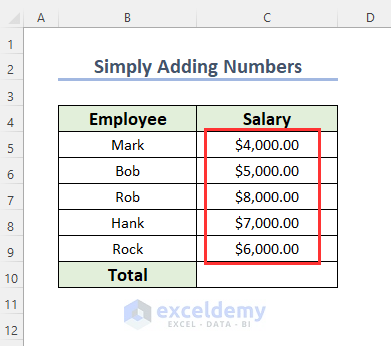
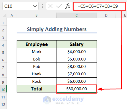
We’ll change the sheet to contain all employee salaries. We are going to add all the salary cells to get the total salary in Cell C10.

Steps:

• Select Cell C10 and type the Equal (=) sign.
• Click on the first cell to add and type the Plus (+) sign.
• Click on the second cell and add a plus sign.
• Repeat until you add all cells.

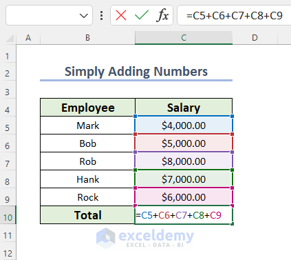
• Press Enter.

Read More: How to Sum Selected Cells in Excel

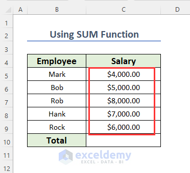
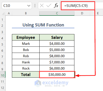
Method 3 – Inserting the SUM Function to Add Multiple Cells in Excel

We’ll get the total salaries of the employees.

Steps:

• Insert “=SUM(“ in Cell C10.
• Select the range of cells that you want to add up.

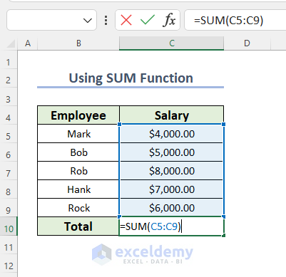
• Press Enter.

Read More: Shortcut for Sum in Excel

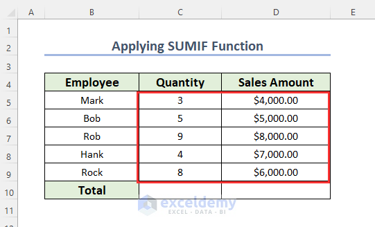
Method 4 – Adding up Multiple Cells with a Condition Using SUMIF Function

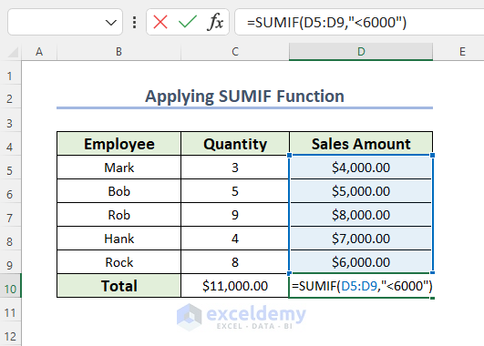
We have a worksheet with some salespeople, their sales quantity, and the sales amount. We are going to add up the sales amount where the quantity is less than 5 and the sales amount that is lower than $6,000.00.

Steps:

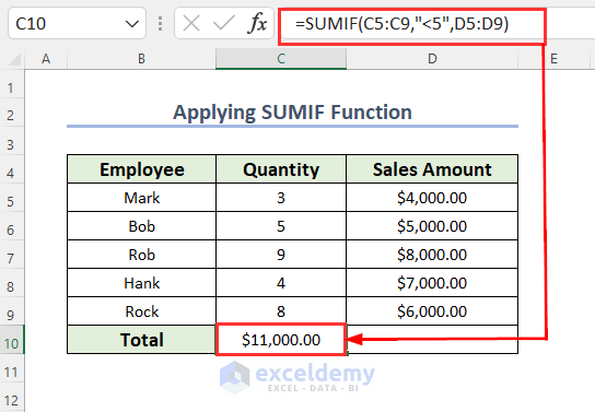
• Use the following formula in cell C10.

Mark, Hank, and Rock have quantities smaller than 5 and so their corresponding sales amount will be added up here.

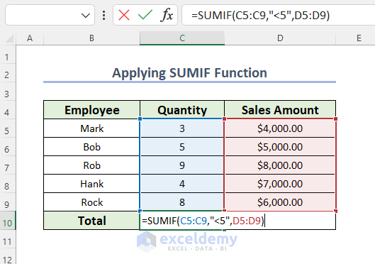
• Press Enter.

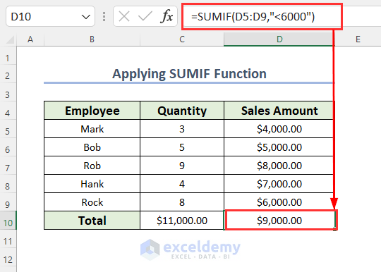
• Insert the following formula in cell D10.

The SUMIF function goes through column D to find the values which are smaller than 6000 and then adds them up.

• Hit Enter.

Read More: Excel Sum If a Cell Contains Criteria

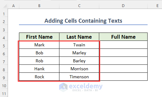
Method 5 – Adding Multiple Cells Containing Texts in Excel

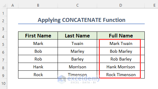
We will add up the cells of the First Name column with the cells of the Last Name column to form the full names in the Full Name column.

Case 5.1 – Applying the CONCATENATE Function

Steps:

• Use the following formula in cell D5.

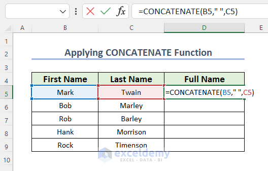
• Press Enter.
• Drag down the Fill Handle tool.

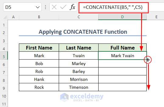
• You will get all of the full names of the employees.

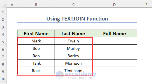
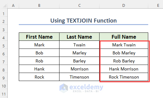
Case 5.2 – Applying the TEXTJOIN Function

We’ll use the same dataset.

Steps:

• Use the following formula in cell D5 and press Enter.

Here, ” ” is the separator of each text, TRUE is for ignoring blank cells, and B5 and C5 are the texts.

• Drag down the Fill Handle tool.

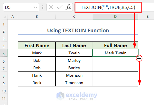
• You will get the combined texts in the Full Name column.

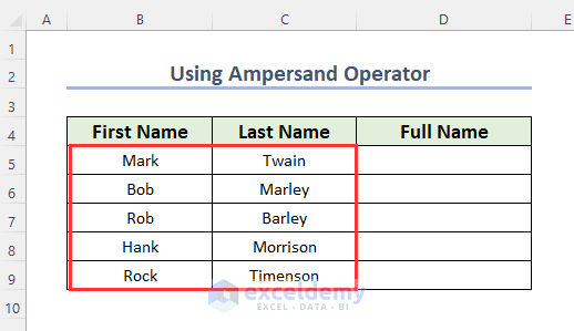
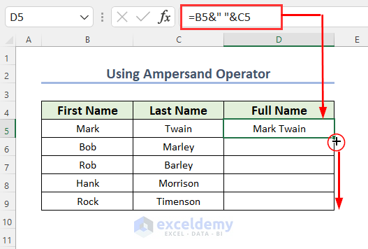
Case 5.3 – Using the Ampersand Operator

We will get the full names by combining the two parts of the names using the Ampersand operator.

Steps:

• Use the following formula in cell D5 and press Enter.

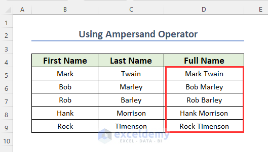
• Drag down the Fill Handle tool.

• You will get the full names.

Read More: Sum If a Cell Contains Text in Excel

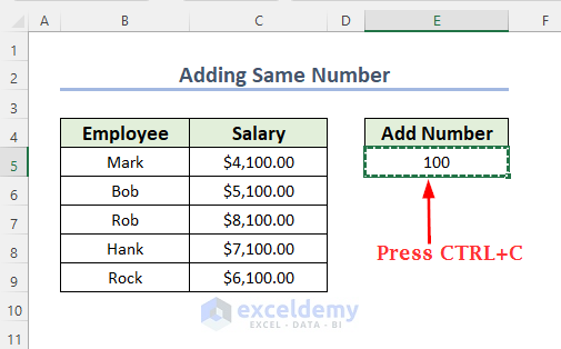
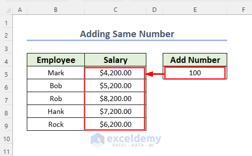
Method 6 – Adding a Constant Number to Multiple Cells Simultaneously

We are going to add the value in cell E5 to multiple cells of the Salary column.

Steps:

• Select Cell E5 and copy it by pressing Ctrl + C.

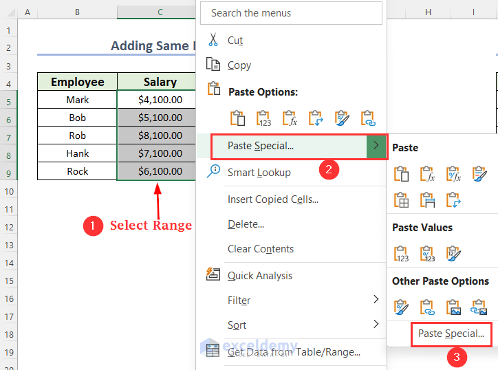
• Select the cells where you want to add the copied values and right-click.
• Click on the arrow symbol next to Paste Special and click on Paste Special again to see more options.

• The Paste Special dialog box will appear.
• Select Values and, in the Operation section, select Add.
• Click OK.

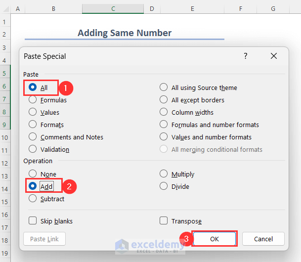
You can also open up this dialog box by pressing Ctrl + Alt + V.

• We can see that 100 has been added to all of the salaries.

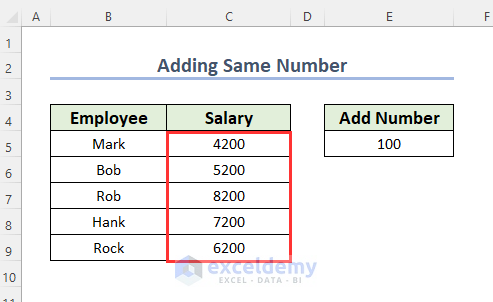
• Apply the Currency format again to get the following outlook.

Read More: How to Add Numbers in Excel

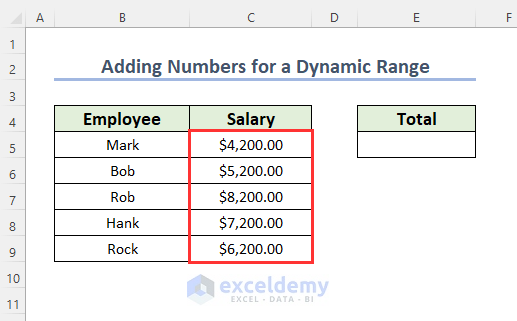
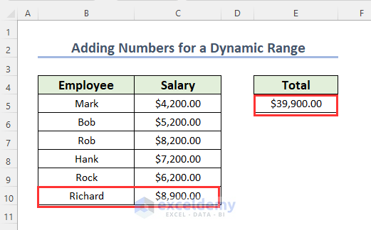
Method 7 – Adding Values of Multiple Cells for a Dynamic Range

We will add up the values of the Salary column in such a way that if we add an extra cell in this column then the value will be automatically added up in the final result.

Steps:

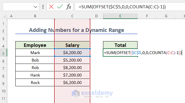
• Use the following formula in Cell E5.

$C$5 is the starting cell of the range, while the following 2 zeros are indicating that the cell reference will not move by any row or column number. COUNTA(C: C)-1 indicates the height number of the range which will be the number of rows having texts or numbers.
The OFFSET function will return the dynamic range and the SUM function will add up them.

• Press Enter.

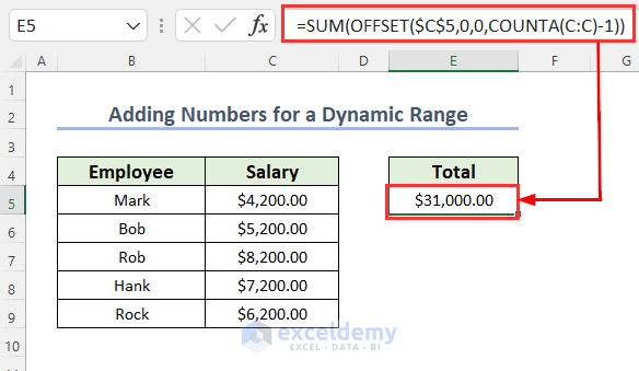
• If we add an extra row for the salary of an employee named Richard, the total value has been automatically changed to $39,900.00.

Read More: How to Sum Range of Cells in Row Using Excel VBA

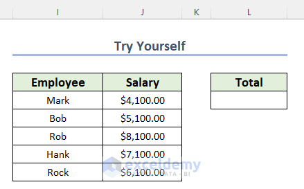
Practice Section

We have created a Practice section on the right side of each sheet so you can test these methods.

Download the Practice Workbook

Related Readings

• How to Sum Colored Cells in Excel
• Use VLOOKUP with SUM Function in Excel
• Sum If Cell Contains Specific Text in Excel
• How to Sum a Column in Excel
• How to Sum Values by Day in Excel