How to Sum Rows in Excel (9 Easy Methods)

Download the Practice Workbook

You can download the practice workbook from here.

Sum Rows.xlsx

9 Quick Methods to Sum Rows in Excel

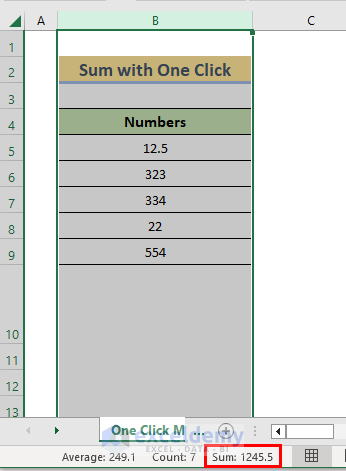
Method 1 – Sum Rows with One Click in Excel

Select column B and look at the Excel Status Bar. You will find the sum there.

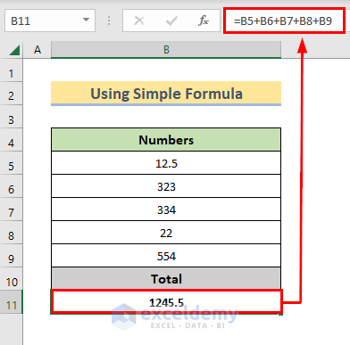
Method 2 – Use a Simple Formula to Sum Rows

Use the following formula in Cell B11 and press Enter.

=B5+B6+B7+B8+B9

We will see the sum value of Cell range B5:B9 in Cell B11.

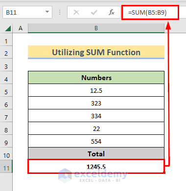
Method 3 – Utilize the SUM Function to Add Rows

Case 3.1 – Add Multiple Rows to a Single Cell

Insert the following formula in Cell B11.

=SUM(B5:B9)

Press Enter.
We will see the sum of elements from Column B in Cell B11.

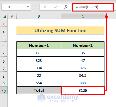
Instead of a single column, we can also sum up a range of cells.

Insert the following formula in Cell C10 and press Enter.

=SUM(B5:C9)

We will see the sum of the range B5:C9 in Cell C10.

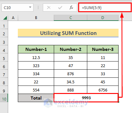
We can adjust the last formula a bit for taking more numbers from entire rows. The adjusted formula is given below:

=SUM(5:9)

We can add more numbers in those rows and the value will be added in Cell C10.

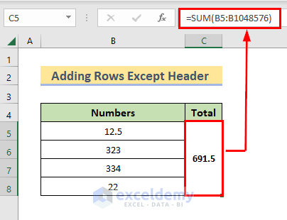
Case 3.2 – Add up Rows Except for Header

Insert the following formula in Cell C5.

=SUM(B5:B1048576)

Press Enter.

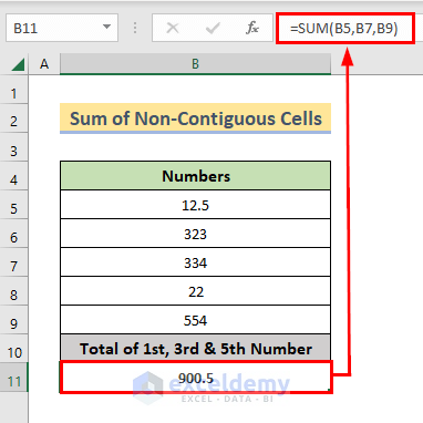
Case 3.3 – Adding Non-Contiguous Cells

Use the following formula in Cell B11.

=SUM(B5,B7,B9)

Hit Enter and you’ll get the sum of values from Cells B5, B7, and B9 in Cell B11.
You can use different cell references to get their sum value.

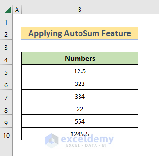
Method 4 – Apply the AutoSum Feature to Sum Rows

Select Cell B10 (or wherever you want the sum of the cells of the same column).
Go to the Formula tab, select AutoSum, and choose Sum.

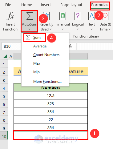
You’ll get the sum of cells above Cell B10.

Similar Readings

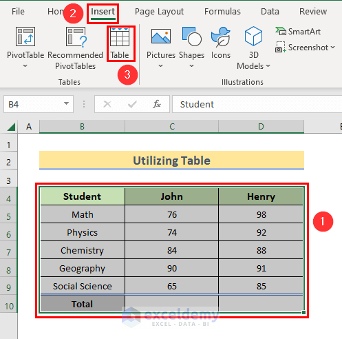
Method 5 – Sum Multiple Rows Utilizing a Table in Excel

Select the whole range of dataset.
Go to the Insert tab and select Table.

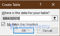
A Create Table window will appear. Hit OK.

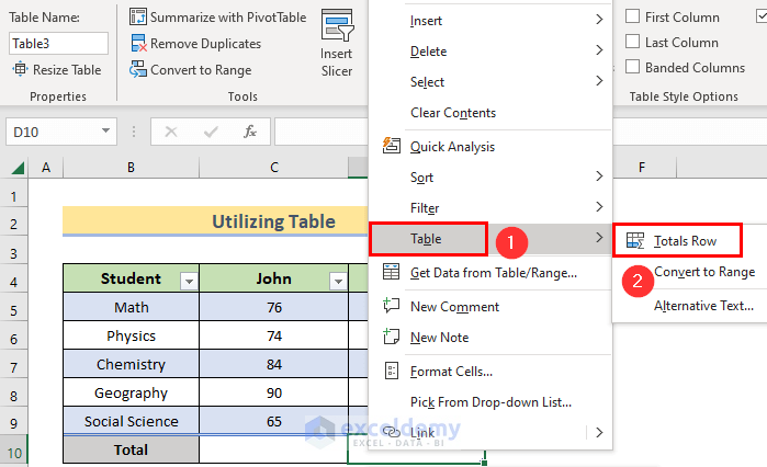
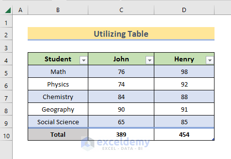
Select Cell D10 to get the sum value there. Right–click on it.
Select Table and choose Total Rows from the context menu.

The sum for Column D is already done.
Move to Cell C10 and click on the small drop-down icon.
Select Sum from the options.

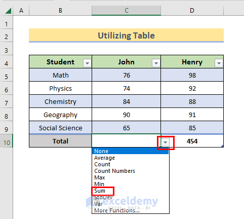
We will get the total sum value of Column C there.

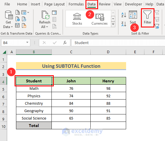
Method 6 – Sum Filtered Rows Using the SUBTOTAL Function in Excel

Select any of the header cells.
Go to the Data tab and select Filter.

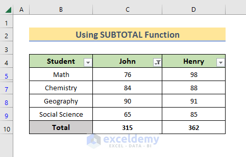
Use the following formula in Cell C10 and press Enter.

=SUBTOTAL(9,C5:C9)

We will see the sum of the range C5:C9 in that cell.

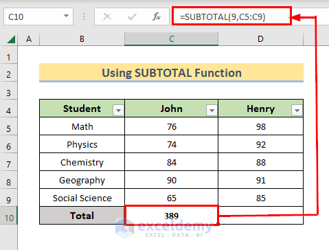
Note: In the argument of the SUBTOTAL function we used 9 which indicates the SUM function.

We can similarly get the sum value of Column D.
Select the filter icon in the header and deselect any number of the column.

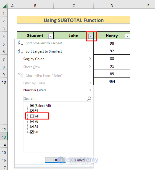
We will get the adjusted result without the deselected value.

Method 7 – Combine SUM, ROW, and MOD Functions to Sum Every K-th Row

Let’s add every second value.

Copy the following formula in Cell B15 to get the sum value there.

=SUM(B5:B14*MOD(ROW(B5:B14),2))

Press Enter.

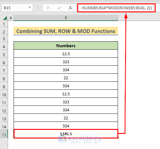
Note: In the formula, we can insert any other number (K) instead of 2 as the argument of the MOD function and we will see the sum of every K-th value from the range.

Method 8 – Apply SUM and LARGE Functions to Sum Higher Values

Use the following formula in Cell B15 and press Enter.

=SUM(LARGE(B5:B14,{1,2,3,4,5}))

We’ll get the sum of the 5 largest numbers from the range.

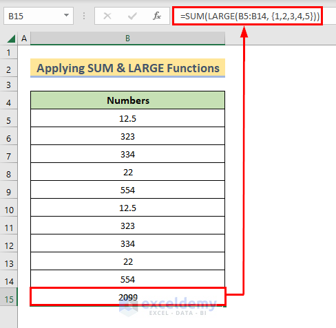
Note: We can change the number of the largest numbers by changing the array {1,2,3,4,5} with more or fewer numbers. For example, if you want to get 3 largest numbers, then you can use {1,2,3} instead.

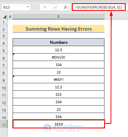
Method 9 – Sum Rows with Errors in Excel

Use the following formula in Cell B15 as we want the sum value there.

=SUM(IFERROR(B5:B14,0))

Press Enter.
We will see the sum of the range B5:B14 while avoiding the cells with errors.