Download the Practice Workbook
3 Methods to Sum Top N Values in Excel
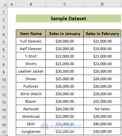
Let’s sum up the top 5 sales from January in the sample dataset.
Method 1 – Combine the LARGE Function with SUMIF to Sum Top N Values in Excel
Steps:
- Insert the following formula in cell F5 and press the Enter key.
=SUMIF(C5:C17,">="&LARGE(C5:C17,5))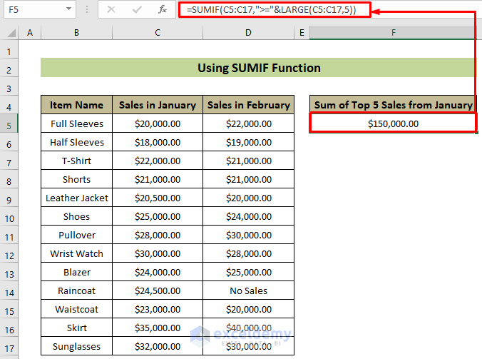
Formula Breakdown:
- LARGE(C5:C17,5)
It returns the 5th largest value from the cells C5 to C17.
Result: $25000.00
- SUMIF(C5:C17,”>=”&LARGE(C5:C17,5))
It returns the sum of the cells from C5 to C17 which contain values greater than or equal to the previous result.
Result: 150,000.00
Thus, you will get the sum of the top 5 sales from January, which is $150,000.00.
Read More: Excel Sum If a Cell Contains Criteria (5 Examples)
Method 2 – Use SUM Formulas to Sum Top N Values in Excel
Case 2.1 – Combine SUM, IF, and RANK Functions to Sum First N Numbers
Steps:
- Insert the following formula in cell F5.
=SUM(IF(RANK(C5:C17,C5:C17)<=5,C5:C17,0))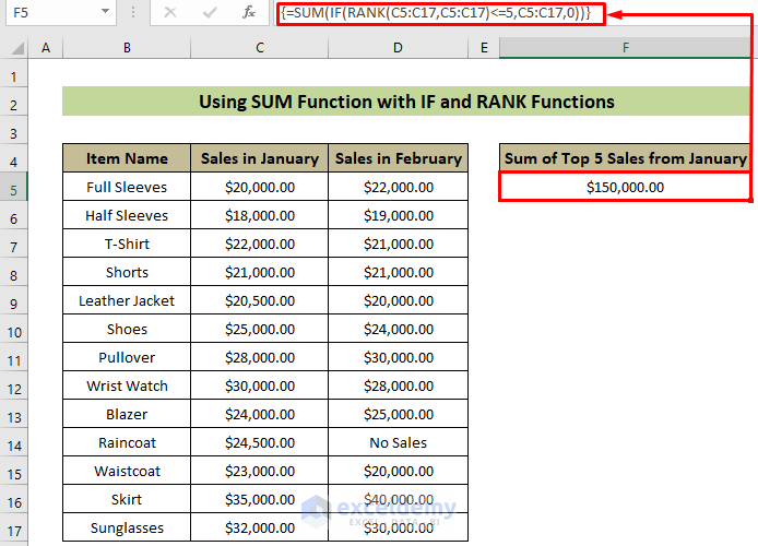
Formula Breakdown:
- IF(RANK(C5:C17,C5:C17)<=5,C5:C17,0)
It takes an array of criteria (RANK(C5:C17,C5:C17)<=5) in place of a single criterion, and it returns a TRUE for each cell between C5 to C17, if it has a value in the top 5 zones. Otherwise, it returns a FALSE. When TRUE, it would return the corresponding cell value from C5 to C17, and when FALSE, it would return 0.
Result: {0,0,0,0,0,25000,28000,30000,0,0,0,35000,32000}
- SUM(IF(RANK(C5:C17,C5:C17)<=5,C5:C17,0))
It sums up the values of the resultant array.
Result: $150,000.00
- Press Ctrl + Shift + Enter as this is an array formula.
We will get the same result as earlier, $150,000.00
Read More: How to Add Multiple Cells in Excel (6 Methods)
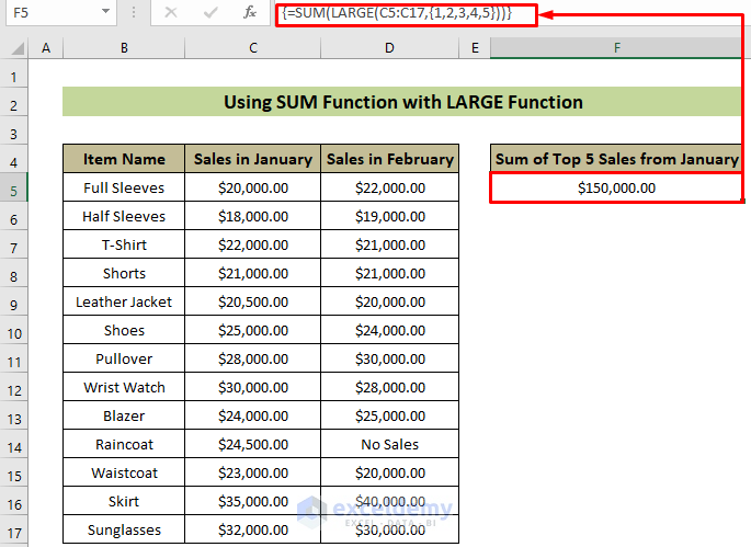
Case 2.2 – Combine SUM with the LARGE Function
Steps:
- Insert the following formula in cell F5.
=SUM(LARGE(C5:C17,{1,2,3,4,5}))- Press Ctrl + Shift + Enter.
Formula Breakdown:
- LARGE(C5:C17,{1,2,3,4,5})
It takes an array of values {1,2,3,4,5} in place of a single value k. And returns an array containing the 1st, 2nd, 3rd, 4th, and 5th largest values from the C5:C17 range.
Result: {35000,32000,30000,28000,25000}
- SUM(LARGE(C5:C17,{1,2,3,4,5}))
It sums up the previous resultant values.
Result: $150,000.00
Consequently, we will get the sum of the top 5 sales from January, which is $150,000.00.
Case 2.3 – Combine SUM with SEQUENCE
We’ll find the sum of the top 10 sales from January this time.
Steps:
- Insert the formula below and hit the Enter key.
=SUM(LARGE(C5:C17,SEQUENCE(10,1)))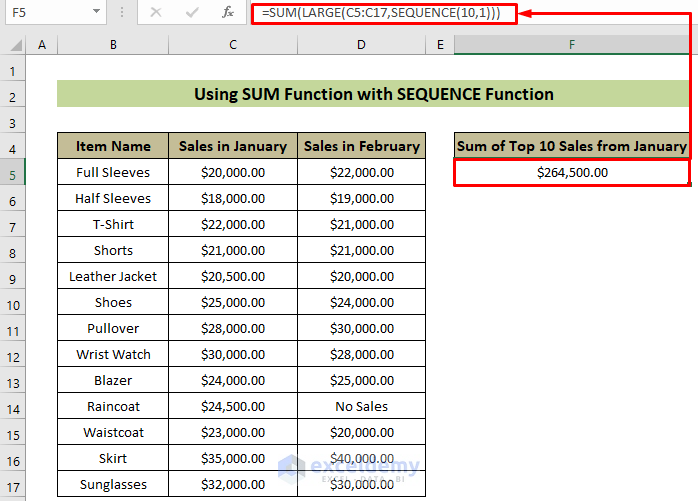
Formula Breakdown:
- SEQUENCE(10,1)
It returns an array of values from 1 to 10.
Result: {1,2,3,4,5,6,7,8,9,10}.
- LARGE(C5:C17,SEQUENCE(10,1))
Returns the top 10 large sales in the range of C5 to C17.
Result: {35000,32000,30000,28000,25000,24500,24000,23000,22000,21000}
- SUM(LARGE(C5:C17,SEQUENCE(10,1)))
Sums the previous resultant array.
Result: $264,500.00
We will get the sum of the top 10 sales of January, which is $264,500.00.
Note:
The SEQUENCE function is only available in Office 365.
Read More: How to Sum Range of Cells in Row Using Excel VBA (6 Easy Methods)
Similar Readings
- How to Add Numbers in Excel (2 Easy Ways)
- All the Easy Ways to Add up (Sum) a column in Excel
- How to Sum Multiple Rows and Columns in Excel
- [Fixed!] Excel SUM Formula Is Not Working and Returns 0 (3 Solutions)
- How to Sum Filtered Cells in Excel (5 Suitable Ways)
Method 3 – Use SUMPRODUCT Formulas to Sum Top N Values in Excel
Case 3.1 – SUMPRODUCT with LARGE, ROW, and INDIRECT Functions
We will get the sum of top 10 sales from January.
Steps:
- Click on cell F5.
- Insert the formula below and press the Enter key.
=SUMPRODUCT(LARGE(C5:C17,ROW(INDIRECT("1:10"))))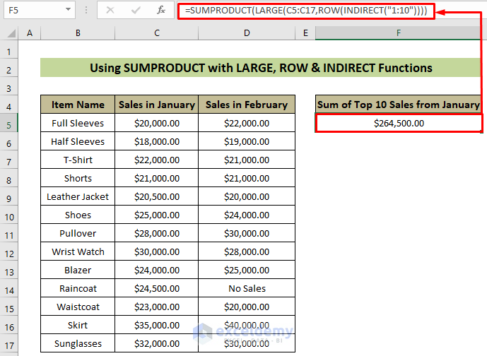
Formula Breakdown:
- ROW(INDIRECT(“1:10”))
It returns an array of values from 1 to 10.
Result: {1,2,3,4,5,6,7,8,9,10}.
- LARGE(C5:C17,ROW(INDIRECT(“1:10”)))
It returns the top 10 large values in range C5 to C17.
Result: {35000,32000,30000,28000,25000,24500,24000,23000,22000,21000}
- SUMPRODUCT(LARGE(C5:C17,ROW(INDIRECT(“1:10”))))
It returns the sum of the top 10 large values.
Result: $264,500.00
Thus, we will get the same result for the top 10 sales of January as earlier, $264,500.00.
Read More: How to Add Rows in Excel with Formula (5 ways)
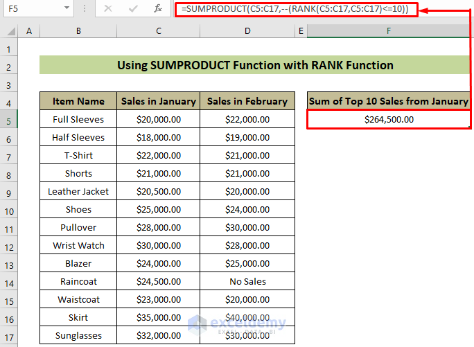
Case 3.2 – SUMPRODUCT with RANK Function
Steps:
- Click on cell F5 and insert the following formula.
=SUMPRODUCT(C5:C17,--(RANK(C5:C17,C5:C17)<=10))- Press the Enter key.
Formula Breakdown:
- –(RANK(C5:C17,C5:C17)<=10)
It returns an array of TRUE or FALSE. For each cell in the range C5 to C17 which falls under the top 10 it returns a TRUE, and FALSE for the rest.‘–‘ converts the TRUE and FALSE array into an array of 1 and 0.
Result: {0,0,1,1,0,1,1,1,1,1,1,1,1}
- SUMPRODUCT(C5:C17,–(RANK(C5:C17,C5:C17)<=10))
It multiplies C5:C17 cell values to the previous resultant array. Therefore, it returns the sum of the top 10 sales.
Result: $264,500.00.
We will get the sum of the top 10 sales values from January.
Read More: Excel Sum Last 5 Values in Row (Formula + VBA Code)
How to Sum Top N Values in Excel with Criteria
We will consider only the top 10 sales below $30,000.00.
Steps:
- Click on cell F5.
- Insert the formula below.
=SUMPRODUCT(C5:C17,(--(RANK(C5:C17,C5:C17)<=10))*(--(C5:C17<30000)))- Hit the Enter key.
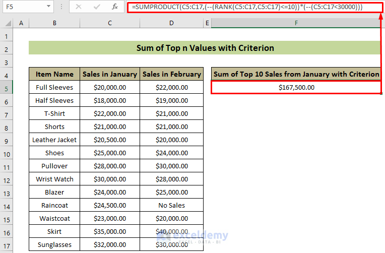
You will get the sum of the top 10 sales in January less than $30,000.00 is $167,500.00 as your desired result.
Note:
You can also use the more complicated formula below:
=SUMPRODUCT(((LARGE(C4:C18,ROW(INDIRECT("1:10"))))<30000)*LARGE(C4:C18,ROW(INDIRECT("1:10"))))
Read More: Sum Cells in Excel: Continuous, Random, With Criteria, etc.
How to Sum Top N Values in Excel with Texts Inside
In a few cells in the February column, there is a text “No Sales”. When we use the formulas from above, it will show errors.
Steps:
- Click on cell F5 and insert the following formula.
=SUM(IFERROR(LARGE(D5:D17,ROW(INDIRECT("1:10"))),0))- Press Ctrl + Shift + Enter.
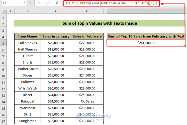
The error because of text calculation will be ignored and you will get the top 10 sales from February would be $261,000.00.
Note:
You can use any other formula from section 2, just wrap the LARGE portion within an IFERROR function.
Read More: How to Sum Cells with Text and Numbers in Excel (2 Easy Ways)
Further Readings
- How to Sum Selected Cells in Excel (4 Easy Methods)
- Sum If a Cell Contains Text in Excel (6 Suitable Formulas)
- How to Sum Only Visible Cells in Excel (4 Quick Ways)
- Sum Only Positive Numbers in Excel (4 Simple Ways)
- How to Calculate Cumulative Sum in Excel (9 Methods)
- Sum Between Two Numbers Formula in Excel
- How to Sum If Cell Contains Specific Text in Excel (6 Ways)

