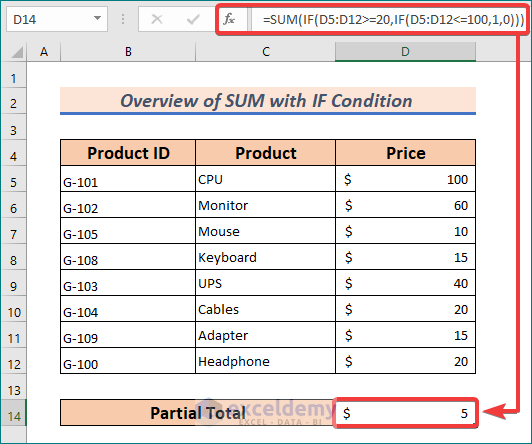
Here’s an overview of using the SUMIF function to check how many values fulfill a condition.
Download the Practice Workbook
The SUMIF Function – an Overview
Sum up a range of cells if the cells meet a given condition.
Syntax
SUMIF(range,criteria,sum_range)
Arguments
- range: This field is mandatory. It refers to the range of cells that include the criteria.
- criteria: This field is also mandatory. It refers to the condition that must be satisfied.
- sum_range: This is an optional requirement. It refers to the range of cells to add if the condition is satisfied.
6 Ways to SUM with the IF Condition in Excel
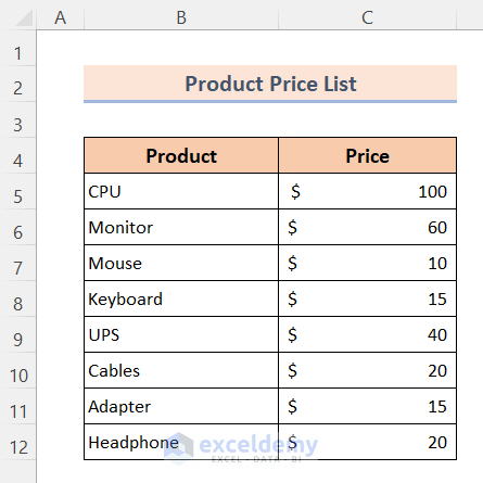
We will be using a sample product price list as a dataset to demonstrate all the methods.
Method 1 – Use SUMIF for Different Comparison Criteria in Excel
Let’s sum up the prices greater than $40.
- Insert the following formula into C14 and hit Enter.
=SUMIF(C5:C12, ">40")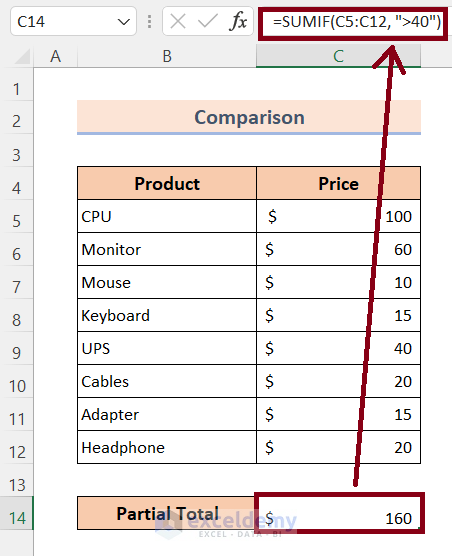
Into the Formula
Within the criteria field, we’ve inserted “>40“, where the “>” operator filters out all the prices greater than $40. As a whole the formula above sums up all the prices greater than $40. There are more operators like the “>” that are listed below:
| Operator | Condition |
| > | Sum if greater than |
| < | Sum if less than |
| = | Sum if equal to |
| <> | Sum if not equal to |
| >= | Sum if greater than or equal to |
| <= | Sum if less than or equal to |
Method 2 – SUM If Various Text Criteria Appear in Excel
We will sum up the prices of all CPU products.
- Insert the following formula into C14 and hit Enter.
=SUMIF(B5:B12, "CPU", C5:C12)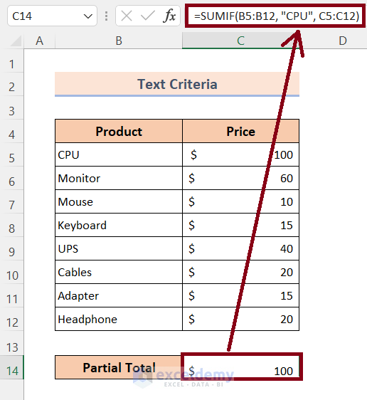
Values based on matches can be split into 2 basic categories:
Case 1 – Exact Match
- Sum for the matched results
=SUMIF(B5:B12, "CPU", C5:C12)- Sum excluding the matched results
=SUMIF(B5:B12, " <>CPU", C5:C12)Case 2 – Partial Match
- Sum for the matched results
Use formula:
=SUMIF(B5:B12, "*CPU*", C5:C12)- Sum excluding the matched results
Use formula:
=SUMIF(B5:B12, " <>*CPU*", C5:C12)Method 3 – Excel SUMIF Function Condition with Numerous Comparison Operators and a Cell Reference
We want to calculate the total prices of all the products excluding the item Monitor.
- In cell C14, we put a value that we’re searching by.
- Insert the following formula into C15 and hit Enter.
=SUMIF(B5:B12,"<>"&C14, C5:C12)
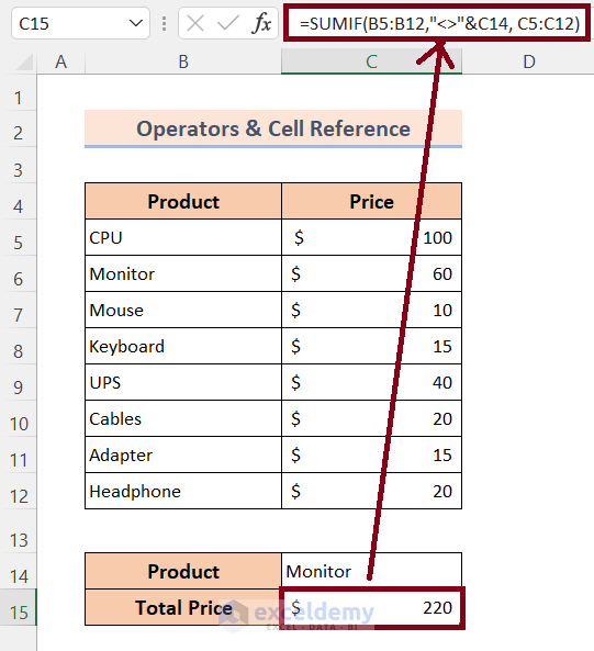
Into the Formula
Within the criteria field, we’ve used “<>”&C14, where the “<>” is responsible for not taking into account what has been pointed out in cell C14.
Case 1 – To sum up prices for the items excluding “Monitor”
=SUMIF(B5:B12,"<>"&C14, C5:C12)Case 2 – To sum up prices for the item “Monitor”
=SUMIF(B5:B12,C14, C5:C12)Method 4 – Use the SUMIF Function Condition with Wildcard Symbols
You can use one of the two wildcard symbols:
- Asterisk (*) – represents any number of characters, including zero.
- Question mark (?) – represents a single character.
Case 4.1 – Partial Matches with Wildcards
1. To sum values that begin with the word “Mouse”
=SUMIF(B5:B12,"Mouse*", C5:C12)2. To sum values that end with the word “Mouse”
=SUMIF(B5:B12,"*Mouse", C5:C12)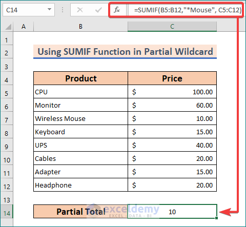
3. To sum values for “Mouse” being present at any position
=SUMIF(B5:B12,"*Mouse*", C5:C12)4. To sum values having at least 1 character present
=SUMIF(B5:B12,"?*", C5:C12)5. To sum values for empty cells
=SUMIF(B5:B12,"*", C5:C12)Case 4.2 – SUM Values Having a Specific Number of Characters
Let’s calculate the total price for products that are three characters long:
- Insert the following formula into C14 and hit Enter.
=SUMIF(B5:B12, "???", C5:C12)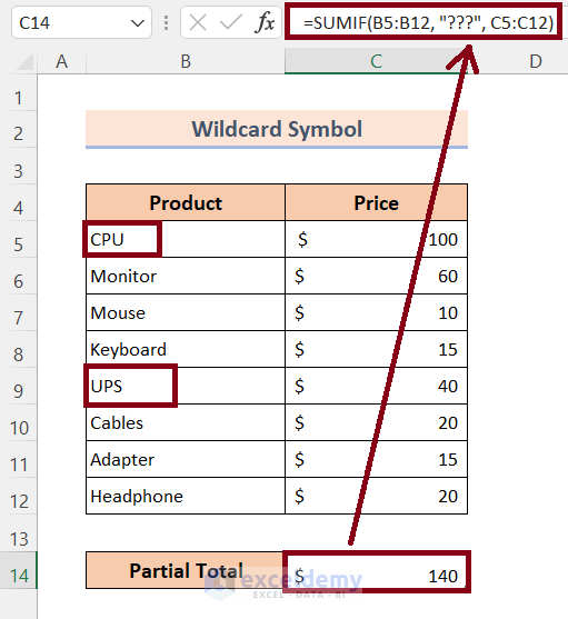
Method 5 – Excel SUMIF Function with a Date Condition
- Insert the following formula into D14 and hit Enter.
=SUMIF(B5:B12,"9/1/2020",D5:D12)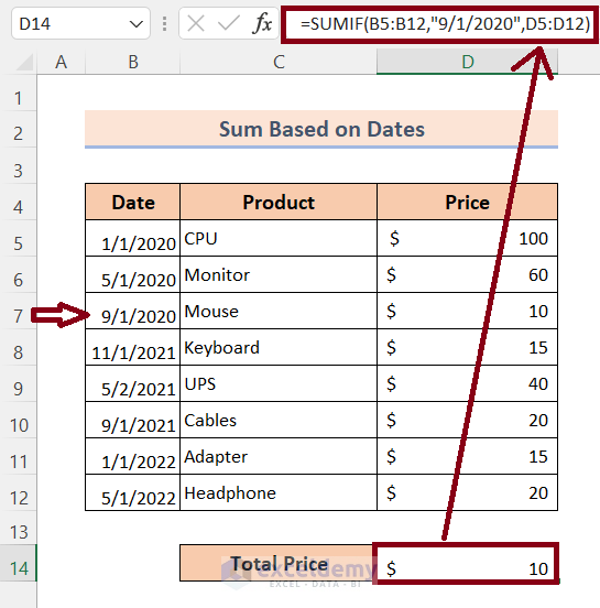
Here are other options you can use:
1. Sum values for current date use
=SUMIF(B5:B12, "TODAY()",D5:D12)2. Sum values before current dates use
=SUMIF(B5:B12, "<"&TODAY(),D5:D12)3. Sum values after current dates use
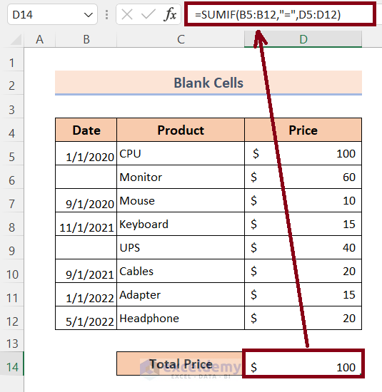
=SUMIF(B5:B12,">"&TODAY(),D5:D12)Method 6 – Sum If Blank Cells Correspond to the Values in Excel
These formulas sum up only those prices whose corresponding dates are missing:
=SUMIF(B5:B12,"=",D5:D12)OR
=SUMIF(B5:B12,"",D5:D12)Both return the same result.
Things to Remember
Be aware of the syntax of the SUMIF function.
Carefully handle the range field inside the formula.
Do not insert arrays in range or sum_range fields.
The size of the range and the sum_range should be the same.
Get FREE Advanced Excel Exercises with Solutions!
