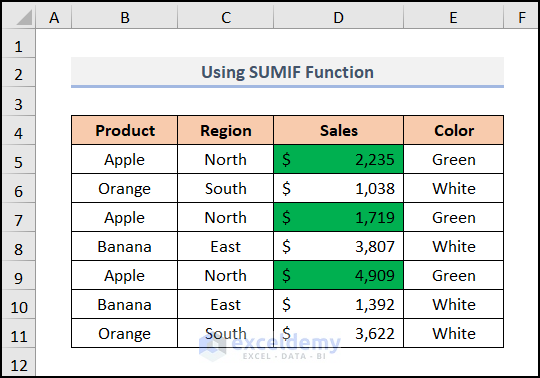
Method 1 – Using SUMIF Function
Steps:
➤ Write the color of cells of the Sales column manually in the Color column.
➤ Select the output cell E12.
➤ Type the following formula.
=SUMIF(E5:E11,"Green",D5:D11)E5:E11 is the criteria_range, Green is the criteria and D5:D11 is the sum_range.
➤ Press ENTER.
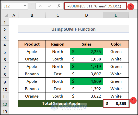
Result:
NGet the Total Sales of Apple which is $8,863.
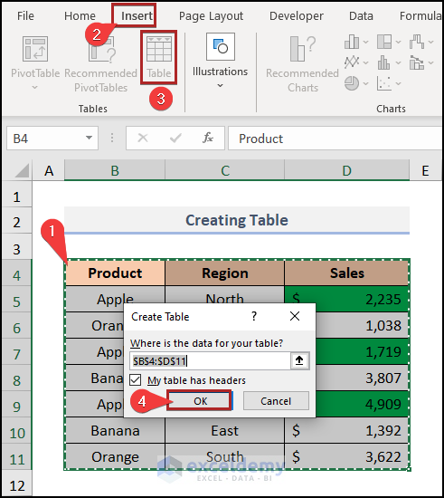
Method 2 – Creating Table to Sum Values of Colored Cells
Steps:
➤ Select the data table (B4:D11).
➤ Go to Insert Tab>>Table Option
The Create Table dialog box will appear.
➤ Click the My table has headers option.
➤ Press OK.
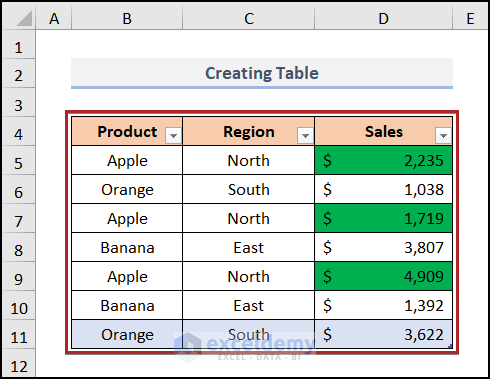
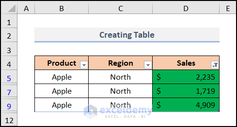
The table will be created.
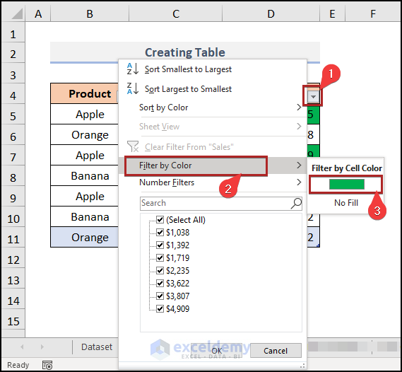
➤Click the Dropdown icon in the Sales column.
➤ Select the Filter by Color option.
➤ Choose the green box as Filter by Cell Color.
➤ Press OK.
The table will be filtered by green.
➤ Select the output cell D12.
➤ Type the following formula.
=SUBTOTAL(109,D5:D9)109 is for the SUM function, and D5:D9 is the range of cells containing Sales.
➤ Press ENTER.
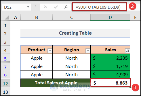
Result:
The Total Sales of Apple is $8,863.
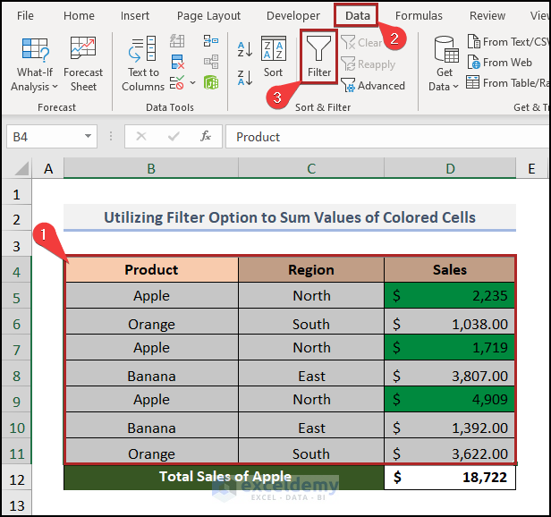
Method 3 – Utilizing Filter Option to Sum Colored Cells
Steps:
➤ Select the output cell D12.
➤ Type the following formula
=SUBTOTAL(109,D5:D11)109 is for the SUM function, and D5:D11 is the range of cells.
➤ Press ENTER.
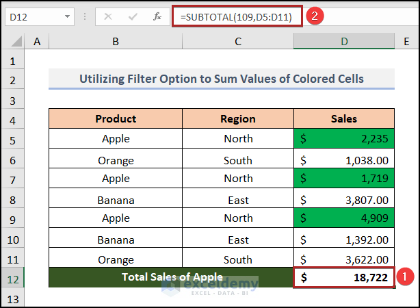
Then, you will get the total Sales.
➤ Select the data range.
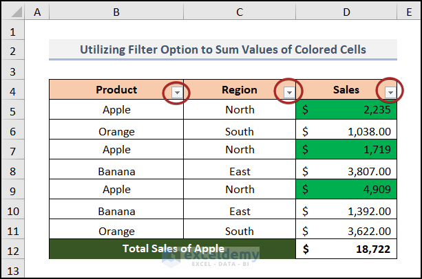
➤ Go to Data tab>>Sort & Filter dropdown>> Filter option.
You can see filter buttons beside each column heading.
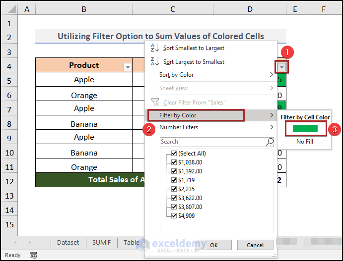
➤ Click the Dropdown icon in the Sales column.
➤ Select the Filter by Color option.
➤ Choose the green box as Filter by Cell Color.
➤ Press OK.
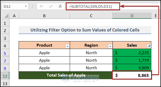
Result:
The Total Sales of Apple is $8,863.
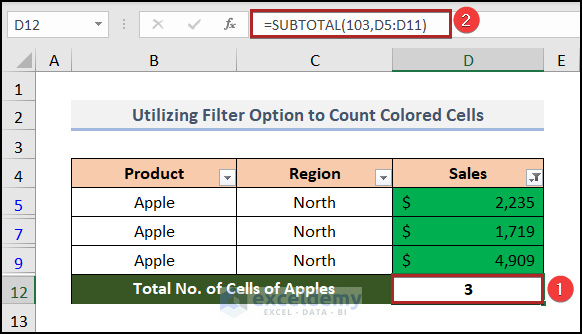
3.2 Count of Colored Cells
Steps:
➤ Select the output cell D12.
➤ Type the following formula.
=SUBTOTAL(103,D5:D11)103 is for the COUNTA function, and D5:D11 is the range of cells.
➤ Press ENTER.
You will get the sum of the total number of cells.
➤ Follow the previous steps of Method-3.1.
You will get the sum of the number of Green colored cells.
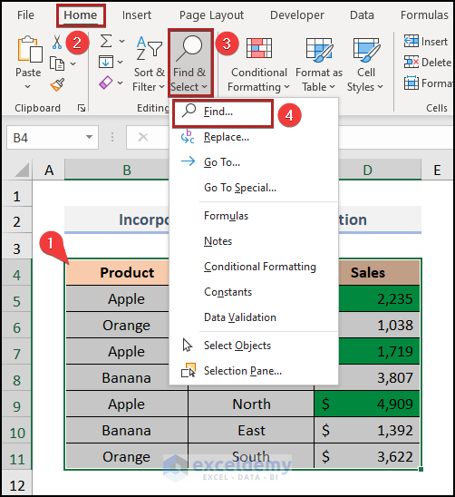
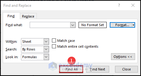
Method 4 – Incorporating Find & Select Option
Steps:
➤ Select the data table (B4:D11).
➤ Go to Home tab>>Editing dropdown>>Find & Select dropdown>>Find option.
After that, the Find and Replace dialog box will pop up.
➤ Select the Format option.
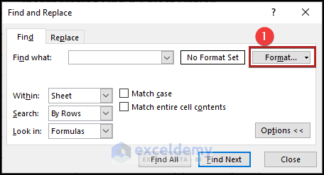
The Find Format dialog box will appear
➤ Select the Fill tab and choose the Green color.
➤ Press OK.
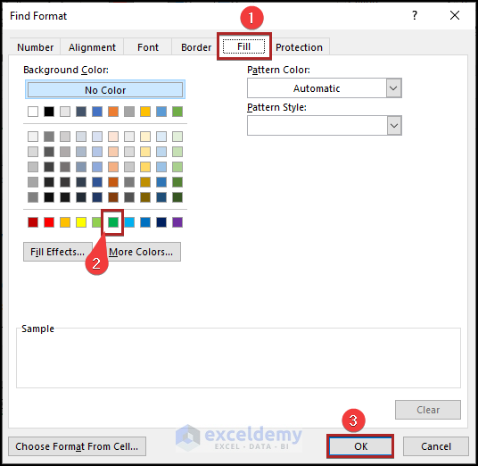
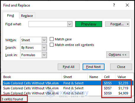
➤ Click Find All.
Result:
The total number of Green colored cells is in the bottom corner of the dialog box, which indicates that there is a total of 3 green colored cells.
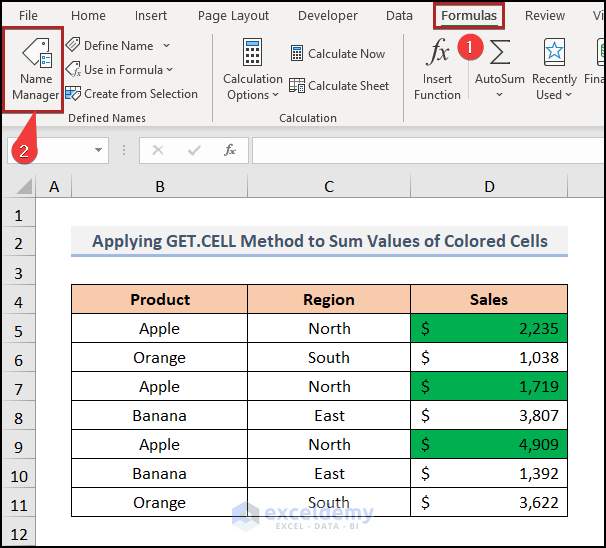
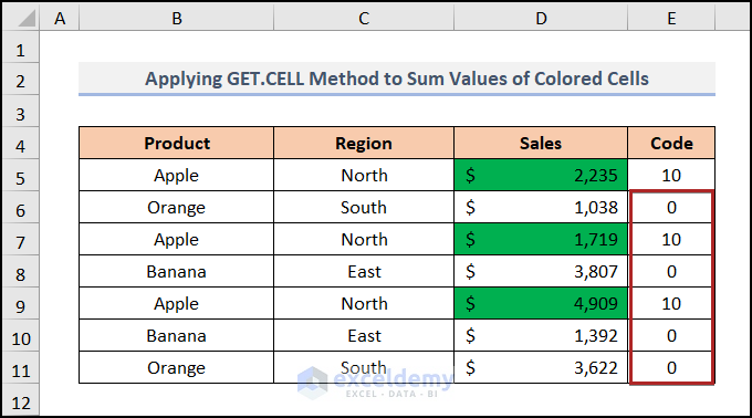
Method 5 – Applying GET.CELL Method
5.1 Sum Values of Colored Cells
The GET.CELL function to sum up the Sales for Green colored cells.
Steps:
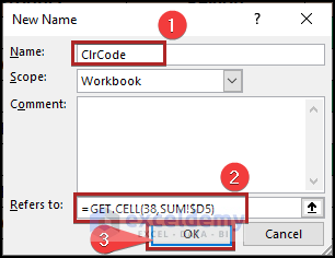
➤ Go to Formulas tab>>Defined Names dropdown>>Name Manager option.
The Name Manager Wizard will appear.
➤ Select the New option.
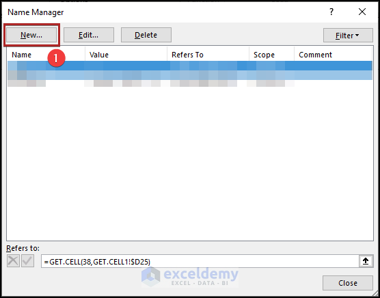
After that, the New Name dialog box will pop up.
➤ Type any type of name in the Name box, here I have used ClrCode.
➤ Select the Workbook option in the Scope box.
➤ Type the following formula in the Refers to box.
=GET.CELL(38,SUM!$D5)38 will return the Color Code and SUM!$D5 is the colored cell in the SUMIF sheet.
➤ Press OK.
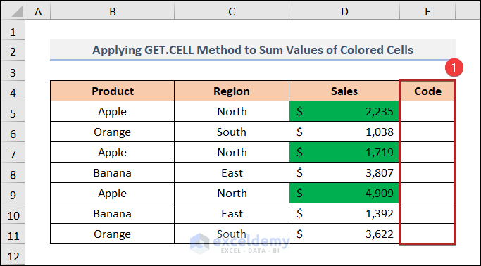
➤ Create a column named Code.
➤ Type the following formula in the output cell E5.
=ClrCode➤ Press ENTER.
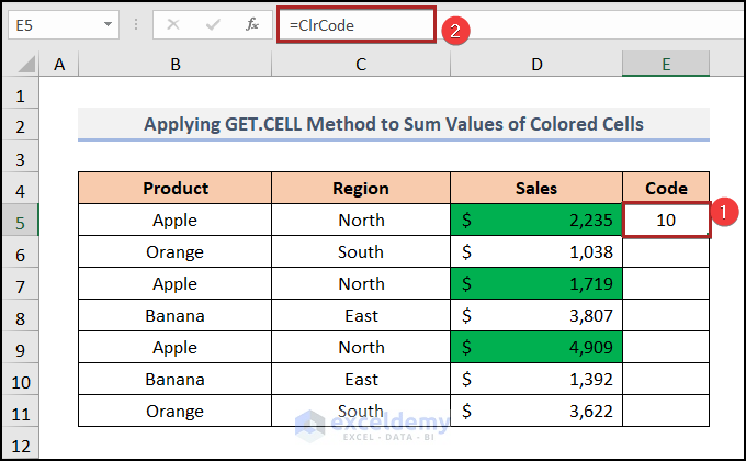
It will return the Code of the colors.
➤ Double-click on the Fill Handle Tool.
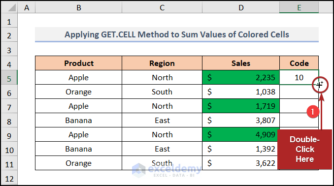
You will get the color codes for all of the cells.
➤ Select the output cell G5.
➤ Type the following formula.
=SUMIF(E5:E11,ClrCode,D5:D11)E5:E11 is the criteria_range, ClrCode is the criteria and D5:D11 is the sum_range.
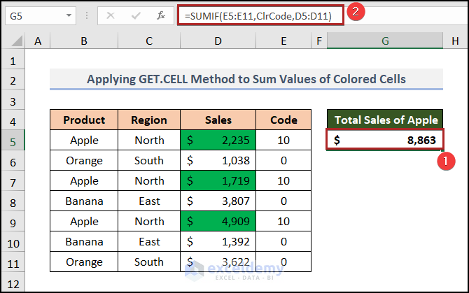
Result:
The Total Sales of Apple is $8,863.
Note: Save the Excel file as a Macro-enabled Workbook because of the GET.CELL function.
5.2 Count of Colored Cells
Steps:
➤ Follow the previous steps of Method-5.1.
➤ Select the output cell G5.
➤ Type the following formula.
=COUNTIF(E5:E11,ClrCode)E5:E11 is the criteria_range, and ClrCode is the criteria.
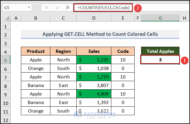
Result:
You will get the total number of Green colored cells in the range.
How to Sum Colored Cells in Excel with VBA
Steps:
➤ Go to the Developer tab >> Visual Basic option.
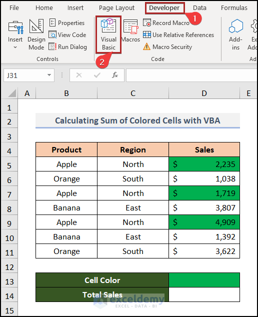
The Microsoft Visual Basic for Applications window will open.
➤ Jump to the Insert tab.
➤ Select Module from the options.
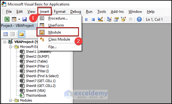
It opens the code module where you need to paste the code below.
Function Sum_Red_Cells(cc As Range, rr As Range)
Dim x As Long
Dim y As Integer
y = cc.Interior.ColorIndex
For Each i In rr
If i.Interior.ColorIndex = y Then
x = WorksheetFunction.Sum(i, x)
End If
Next i
Sum_Red_Cells = x
End Function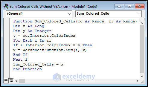
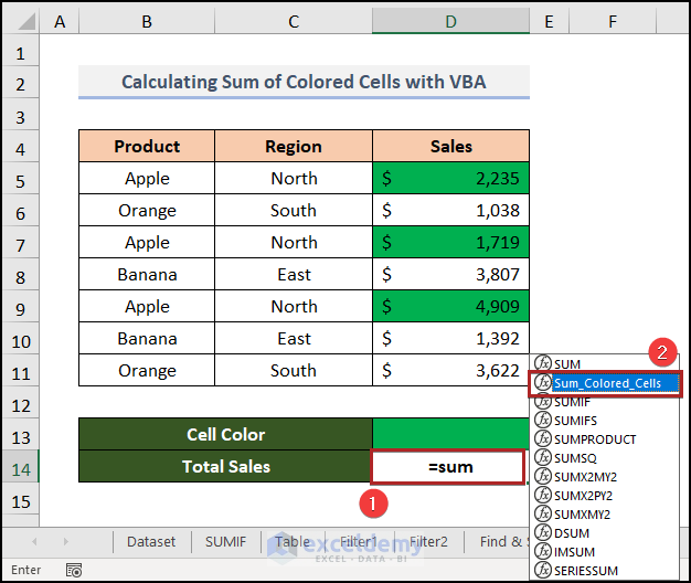
Navigate to the VBA worksheet “VBA”.
➤ Select cell D14 and start to write the function name we just created.
You can see that the function name appears just after writing down =sum in the cell.
➤Select the function Sum_Colored_Cells and press the TAB key on the keyboard.
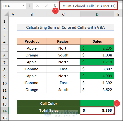
Give the necessary arguments for the function. D13 is the cell reference for the green-colored cell. D5:D11 is the cell range to perform the sum operation.
Download Practice Workbook
You may download the following Excel workbook for better understanding and practice.
Further Readings
- How to Sum Random Cells in Excel
- How to Sum in Excel If the Cell Color Is Red
- [Solved!] Currency Sum Not Working in Excel
- How to Ignore Blank Cells in Excel Sum
<< Go Back to Sum in Excel | Calculate in Excel | Learn Excel
Get FREE Advanced Excel Exercises with Solutions!
