In this article, we will demonstrate five examples of how to efficiently implement Excel VLOOKUP to find the closest match in Excel.
As an example of finding the closest match, suppose we want to find the name of a student who achieved 100 marks on the Math test, but no one achieved that mark. So we will identify the student who achieved the closest mark to 100. With the help of the VLOOKUP function, we can find this student/mark easily.
VLOOKUP Function in Excel: Syntax
Generic formula:
=VLOOKUP(lookup_value, table_array, col_index_num, [range_lookup])Here,
| Arguments | Definition |
|---|---|
| lookup_value | The value to be matched. |
| table_array | The data range in which to lookup the value. |
| col_index_num | The corresponding column from which to return the result |
| range_lookup | This is a Boolean value: TRUE or FALSE. FALSE (or 0) means exact match and TRUE (or 1) means approximate match. |
Things to Remember
To avoid errors, keep the following in mind while working with the VLOOKUP function:
- The data in the lookup table must be sorted in ascending order.
- As the range of the data table array to search for the value is fixed, place dollar ($) signs in front of the cell reference numbers of the array table to make the references absolute.
- When working with array values, press Ctrl + Shift + Enter to return results. Pressing only Enter doesn’t work when using array formulas, except in Office365 version.
With that in mind, let’s see the VLOOKUP function in action.
We will demonstrate how to utilize the VLOOKUP function to find a partial match in text, to find the closest value to a predefined value, to find the commission rate of sales personnel, to find the best candidate for a job, and finally, to find an upcoming event date.
Example 1 – Finding a Partial Match in Text Using VLOOKUP
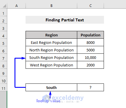
Consider the following data table, where we want to find the population of the “South Region”, but don’t want to write the long name in our search bar. In the indicated lookup box below, we’ll enter a part of the Region name, and in the next cell apply a VLOOKUP formula to return the corresponding Population value.
Our formula is:
=VLOOKUP(B6, $B$5:$C$8, 2, TRUE)Formula Explanation:
The formula looks for -> B6 = South Region Population
In -> $B$5:$C$8 = The Array Data Table.
2 = Returns the value in the same row from the second column of the table array.
TRUE = Returns an approximate match
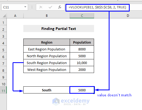
However, the population of the “South Region” is not returned.
The problem is that VLOOKUP performs range-wise, meaning it scans down the first column and returns the row where the value is greater or equal to the row and less than the value in the next row.
Theoretically, the text string “North Region Population” is equal to “South Region Population”, so the value from the “North Region Population” row is returned.
To return an accurate result from a partial-string match, use a character to represent another character. For instance, in the modified formula below, we concatenate our lookup value with an Asterisk (*) using the Ampersand (&) symbol:
=VLOOKUP(B11&"*", $B$5:$C$8, 2, TRUE)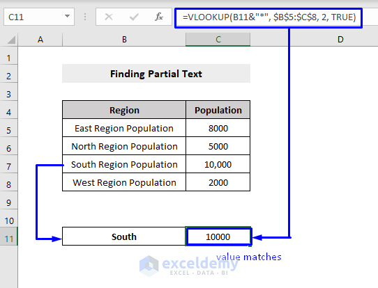
Now, the Population of the “South Region” is correctly returned in the result cell C11.
Read More: How to Use VLOOKUP to Find Partial Text from a Single Cell
Example 2 – Finding the Closest Match to the Lookup Value Using VLOOKUP
Now let’s find the closest match to a certain value in a large dataset using VLOOKUP.
Consider the following data table. Let’s find the closest match to our lookup value, 24.
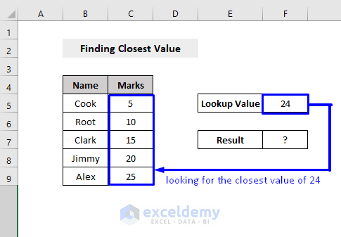
Our formula in cell F5 is:
=VLOOKUP(F5, $C$5:$C$9, 1, TRUE)Explanations:
Look for -> F5 = 24
In -> $C$5:$C$9 = The Array Data Table.
1 = Returns the value from corresponding column number 1.
TRUE = Returns an approximate match.
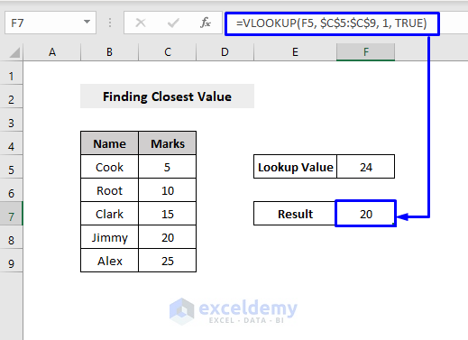
The formula returns 20, not 25, even though 24 is the closest match to 25. Why is that?
VLOOKUP scans down the first column and returns the row where the value is greater or equal to the row and less than the value in the next row.
So, it starts scanning for the highest value less than the value of 24. When it reaches the value 25, it stops the execution and returns the previous row with the closest value, 20, as the result.
Example 3 – Finding the Commission Rate (Looking for the Closest Sales Value) Using VLOOKUP
Consider the following dataset where the commission will be distributed based on the Sales, which is calculated using the table on the right.
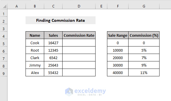
For example, if a salesperson’s Sale Range is around 5000 then the Commission is 0%, if the Sale Range is around 20000 then the Commission is 7%, and so on. To return the Commission Rate, we need to find the closest match to the Sale Range and lower the Sales value.
As an example, for the 16427 Sales value (cell C5), the Commission would be 5%, as it is below the 10000 Sale Range (cell F6). As a result, using the Commission value from the table on the right (cell G6), the Commission Rate becomes 0.05 (cell D5).
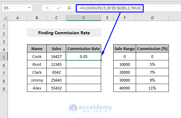
The formula in cell D5 to calculate the commission rate is:
=VLOOKUP(C5,$F$5:$G$9,2, TRUE)Explanation:
Looks for -> C5 = 16427, the Sales value of the salesperson Cook
In -> $F$5:$G$9 = the Array Data Table.
2 = Returns the value in the same row from the second column of the table array.
TRUE = Returns an approximate match.
This calculates the commission rate of the salesperson named Cook and displays the result in cell D5.
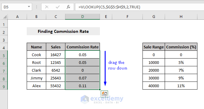
Drag the formula down using the Fill Handle to apply the formula to the rest of the rows.
Example 4 – Selecting the Candidate with the Closest Experience Using VLOOKUP
Excel’s LOOKUP function can be useful for finding the right person for a job.
Consider the following table:
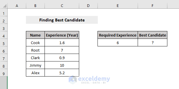
Suppose we want to find the employee who has the work experience closest to the required value, 6 years of work experience in this case.
- Select an empty cell where the employee name will appear and enter the following formula:
=INDEX($B$5:$B$9,MATCH(MIN(ABS(E5-C5:C9)),ABS(E5-$C$5:$C$9),0))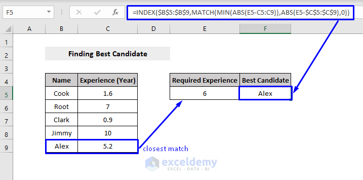
The name of the employee who best fits the job is returned.
Formula Explanation:
E5-$C$5:$C$9 -> The required Experience (6 years) minus the Year of Experience of Each Employee.
Output: 4.4, -1, 5.1, -4, 0.8
This subtracts the Years of Experience of each employee from the Required Experience and returns multiple results because it runs through the whole array table, calculates for every member (Cook, Root, Clark, Jimmy, Alex), and produces the results for all of them.
ABS(E5-$C$5:$C$9) -> The ABS function removes the minus sign (-) from a negative number, making it positive. The ABS function has no effect on 0 (zero) or positive numbers
Output: 4.4, 1, 5.1, 4, 0.8
MIN(ABS(E5-C5:C9)) -> Returns the minimum value from the absolute (ABS) values.
Output: 0.8
MATCH(MIN(ABS(E5-C5:C9)),ABS(E5-$C$5:$C$9),0) -> Finds the position of the 0.8 (first argument in MIN(ABS(E5-C5:C9))) in the array constant (second argument in ABS(E5-$C$5:$C$9)). In this example, we want the MATCH function to return an exact match, so we set the third argument to 0 (or FALSE).
Output: 5
INDEX($B$5:$B$9,MATCH(MIN(ABS(E5-C5:C9)),ABS(E5-$C$5:$C$9),0)) -> The INDEX function takes two arguments to return a specific value in a one-dimensional range. Here, the range $B$5:$B$9 is the first argument, and the result from the calculation in the previous section, position 5, is the second argument. So, we are searching the value located in position 5 in the $B$5:$B$9 range.
Example 5 – Finding the Next Event Date Using VLOOKUP
Suppose, in the following sample data table, we want to know the next upcoming birthday.

We can simply implement an Excel lookup formula to accomplish this.
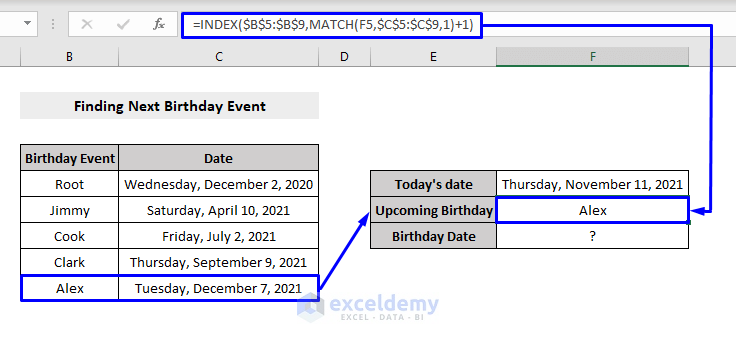
The formula for the person’s name or the upcoming event’s name is:
=INDEX($B$5:$B$9,MATCH(F5,$C$5:$C$9,1)+1)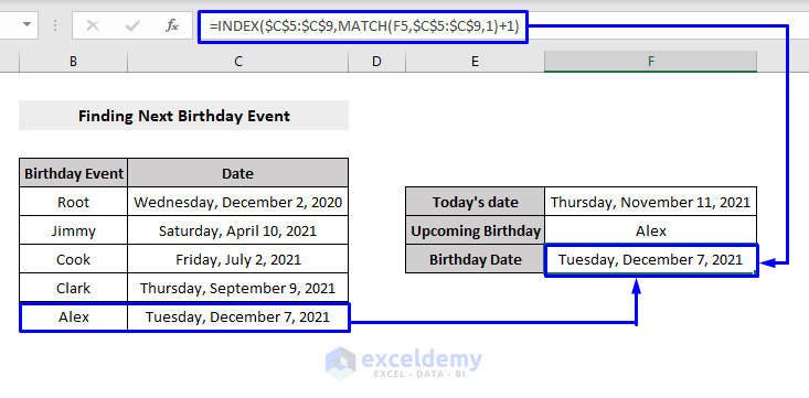
And the formula for the date of the upcoming event is:
=INDEX($C$5:$C$9,MATCH(F5,$C$5:$C$9,1)+1)Formula Explanation:
MATCH(F5,$C$5:$C$9,1) -> Finds the position of the lookup value (cell F5->Thursday, November 11, 2021) in the array constant ($C$5:$C$9 -> the list of the dates). In this example, we want the MATCH function to return an approximate match, so we set the third argument to 1 (or TRUE).
Output: 4
INDEX($B$5:$B$9,MATCH(F5,$C$5:$C$9,1)+1) -> Takes two arguments to return a specific value in a one-dimensional range. Here, the range $B$5:$B$9 is first the argument and the result from the calculation in the previous section (MATCH(F5,$C$5:$C$9,1)), position 4, is the second argument. So, we are searching for the value located in position 4 in the $B$5:$B$9 range.
Output: Alex/(The event’s name)
And,
INDEX($C$5:$C$9,MATCH(F5,$C$5:$C$9,1)+1) -> Takes two arguments to return a specific value in a one-dimensional range. Here, the range to $C$5:$C$9 is the first argument and the result rom the calculation in the previous section (MATCH(F5,$C$5:$C$9,1)), position 4, is the second argument. So, we are searching for the value located in position 4 in the $C$5:$C$9 range.
Output: Tuesday, December 7, 2021
For the upcoming event date, we simply added one to the cell position returned by the MATCH function, to indicate the next column.
Read More: How to Vlookup Partial Match for First 5 Characters in Excel
Download Practice Workbook
Related Articles
- How to Use VLOOKUP to Find Approximate Match for Text in Excel
- How to Perform VLOOKUP with Wildcard in Excel
- Use VLOOKUP to Find Multiple Values with Partial Match in Excel
- Excel VLOOKUP for Partial Match in Table Array
<< Go Back to VLOOKUP Partial Match | Excel VLOOKUP Function | Excel Functions | Learn Excel
Get FREE Advanced Excel Exercises with Solutions!

Need to approximately match addresses on 2 sheets and tell me a job # associated
–sheet 1 has the address (from a trip recorded from fleet software)
–sheet 2 has the job exact address and job # from our CRM
–have a cell to put in the formula to match the addy approximately and find the job # and record it.
Hi Sue,
Hope you are doing well.
You can approximately match addresses on 2 sheets and find a job associated with that address.
Here, we created a dataset in Sheet1 according to your description.
Again, this is Sheet2 containing the exact Address and Job record.
Now, to approximately match addresses on 2 sheets and find a job associated with that address use the formula given below in Sheet1 Cell C5.
=VLOOKUP(B5,Sheet2!$B$5:$C$11,1,TRUE)Thanks.
Regards,
Arin Islam