Example 1 – Using Wildcards in the VLOOKUP Function to Look up a Partially Matched Text
Steps:
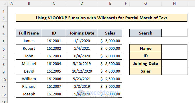
- Prepare the dataset: assign cells to insert the lookup value (here, H4) and cells to see the output (here, H6:H9).
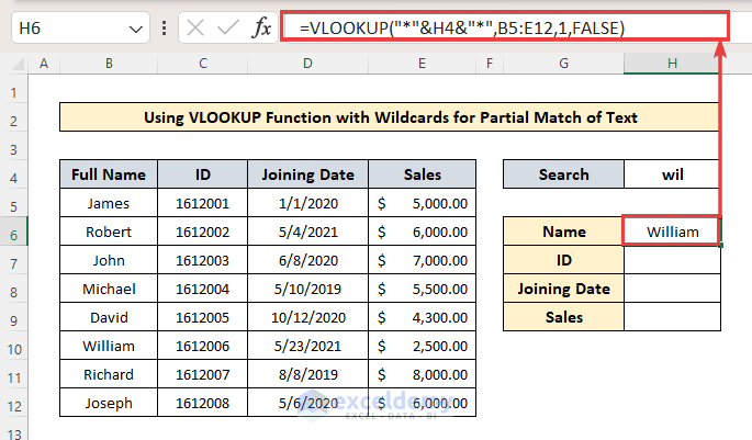
- Enter the formula in H6:
=VLOOKUP("*"&H4&"*",B5:E12,1,FALSE)Formula Breakdown:
Syntax of VLOOKUP Function: =VLOOKUP(lookup_value,table_array,col_index_num,[range_lookup])
- Lookup_value = “*”&H4&”*”: the look_up value is H4 and the asterisk(*) is used before and after the cell reference.
- Table_array = B5:E12: is the table array in which the Vlookup function will work.
- Col_index_num=1: extracts the value of 1st column of the row in which the partial match is found.
- Range_lookup = False: False is used for a Partial Match.
This is the output.
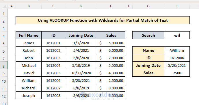
- To see the ID, Joining Date, and Sales value, change the column index number to 2, 3, and 4 in the formula.
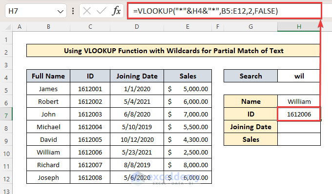
- Enter “wil” in the search box.
This is the output.
Read More: How to Use VLOOKUP to Find Partial Text from a Single Cell
Example 2 – Using the VLOOKUP Function for a Partial Match (the First 3 Characters)
Steps:
- Enter the formula in H6:
=VLOOKUP(LEFT($H$4,3)&"*",$B4:$E$12,1,FALSE)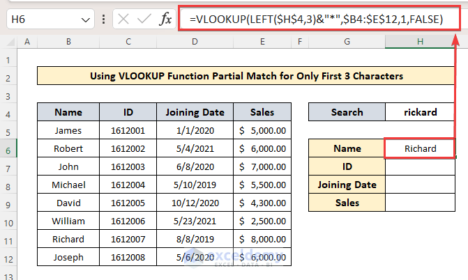
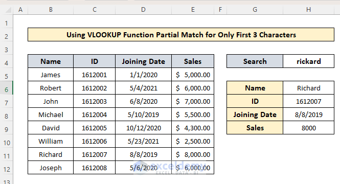
- Change the column index number in the VLOOKUP function to 2, 3, and 4 to see the ID, Date, and Sales values.
Read More: How to Vlookup Partial Match for First 5 Characters in Excel
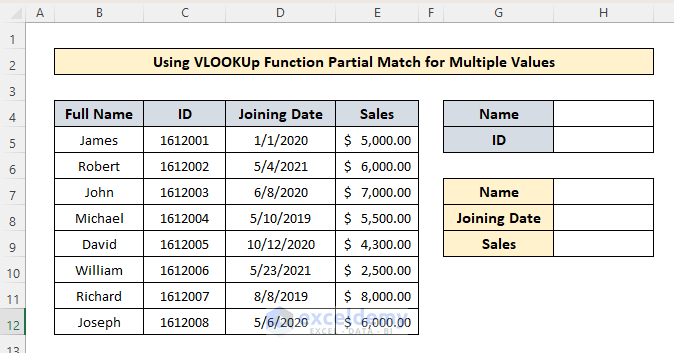
Example 3 – Look Up a Partial Match for Multiple Values
Steps:
- Create search boxes to enter partial names and IDs. Here, H4 and H5.
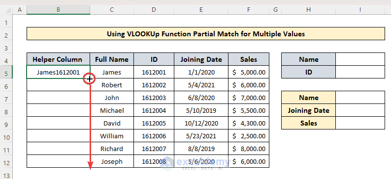
- Insert a helper column to enter the combined text of the the columns “Full Name” and “ID”.
- Enter the formula in B5:
=C5&D5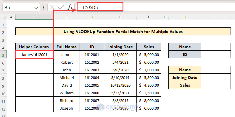
- Drag down the Fill Handle to paste the formula into the other cells or press Ctrl+C and Ctrl+V to copy and paste.
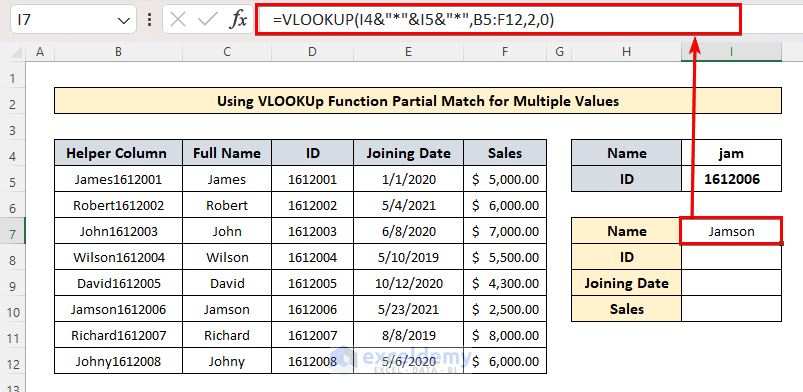
- Enter the formula in I7:
=VLOOKUP(I4&"*"&I5&"*",B5:F12,2,0)Formula Breakdown:
The formula searches for the row values that partially match the values in I5 and I6 and returns the output in the helper column.
- Change the column index numbers to see ID, Joining Date, and Sales.
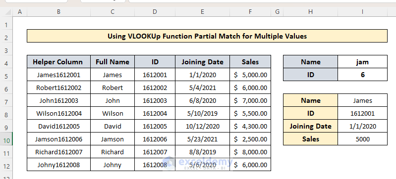
Two names in the “Full Name” column match the search item “Jam”: “James” and “Jamson”. Only “James” is returned as “6” matches James only.
The Excel VLOOKUP Function Does Not Work for Partial Matches in Table Array – Solutions
1. Wrong Placement of Wildcard Characters
Place the Asterisk (*) / wildcard characters between inverted commas. Use an ampersand(&) between the asterisk and the cell reference:
VLOOKUP(“*”&lookup_value&”*”,table_array, column_index_num, [range_lookup])
2. False Column Number Reference in Formula
Recheck the column index number and the table array. The look_up value must be in the first column of the selected data range.
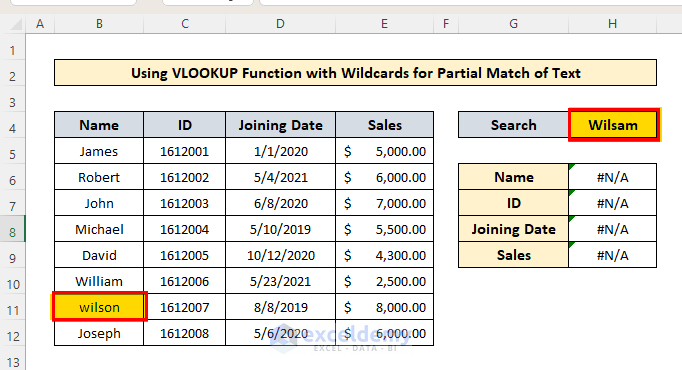
3. Mismatch Between Search and Source Data
You can’t search for an item with extra or different characters from the target value. Observe the image below.
4. Extra Space Inside the VLOOKUP Formula
Remove spacing between symbols and cell numbers.
Download Practice Workbook
Download the practice workbook.
Related Article
- How to Use Excel VLOOKUP to Find the Closest Match
- How to Use VLOOKUP to Find Approximate Match for Text in Excel
<< Go Back to VLOOKUP Partial Match | Excel VLOOKUP Function | Excel Functions | Learn Excel
Get FREE Advanced Excel Exercises with Solutions!
