How to Vlookup a Partial Match for the First 5 Characters in Excel

Why Should We Use VLOOKUP Function for Partial Match?

The VLOOKUP function fetches data from one table to another when the lookup value matches the value of the lookup table. So, even a small space or extra character will give an error value as output such as a not available (#N/A) error. If we want to avoid this error, we need to use a partial match of the lookup value technique with the VLOOKUP function.

Dataset Overview

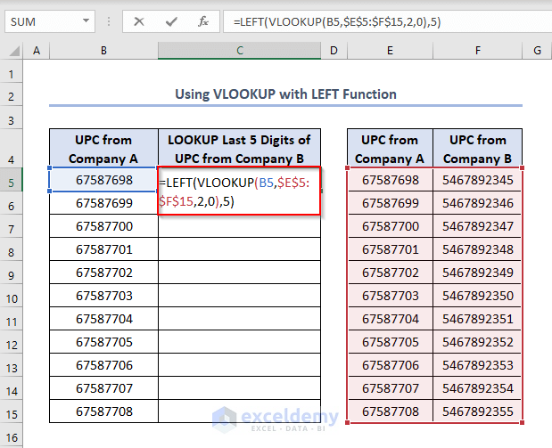
Suppose we have a datasheet named Using VLOOKUP and LEFT functions. Our goal is to find the first 5 characters from the cells in the UPSC column from Company B and display them in the C column.

Step 1 – Insert the VLOOKUP Formula

• In cell C5, enter the following formula:

Here:

• B5 refers to the lookup value (e.g., 67587698, which corresponds to the first UPSC from Company A).
• $E$5:$F$15 is the range where we want to look for the value.
• The 2 indicates that we want to retrieve the second column (which contains the relevant data).
• The 0 specifies an exact match.

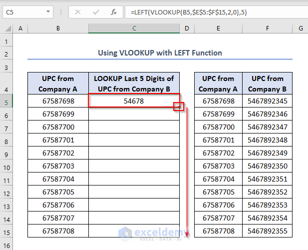
• Press ENTER.
• This formula will return the first 5 characters of the first UPSC from Company B (e.g., 54678).

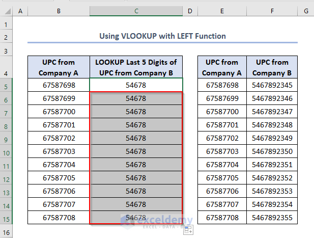
Step 2 – Apply the Formula to Other Cells

• Use the Fill Handle (drag down from the right-bottom corner of cell C5) to apply the formula to other cells in column C.
• This will give you the first 5 characters of the UPSC values from Company B for all relevant rows.

Read More: How to Use VLOOKUP to Find Partial Text from a Single Cell

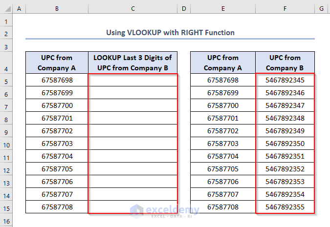
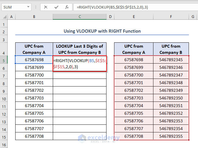
How to Vlookup a Partial Match for the Last 3 Characters

If you want to retrieve the last 3 characters, follow these steps:

Steps:

• Enter the Formula:
  • In cell C5, enter the following formula:

• • • The breakdown remains the same as before.

• •  Press ENTER.
  • This formula will return the last 3 characters of the corresponding UPSC value (e.g., 345).

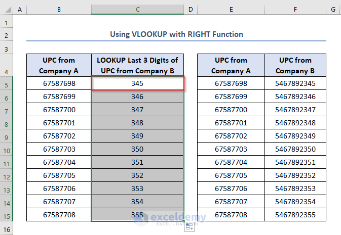
• Apply the Formula:
  • Use the Fill Handle to apply the formula to other cells in column C.
  • You’ll get the last 3 characters of the UPSC values from Company B for all relevant rows.

Read More: Excel VLOOKUP for Partial Match in Table Array

Things to Remember

• Ensure that the lookup value in the table matches the one in the formula cell for the VLOOKUP function to work correctly.
• Otherwise, you may encounter errors while seeking valid output.

Download Practice Workbook

You can download the practice workbook from here:

Related Articles

• Use VLOOKUP to Find Multiple Values with Partial Match in Excel
• How to Use Excel VLOOKUP to Find the Closest Match
• How to Use VLOOKUP to Find Approximate Match for Text in Excel
• How to Perform VLOOKUP with Wildcard in Excel

<< Go Back to VLOOKUP Partial Match | Excel VLOOKUP Function | Excel Functions | Learn Excel