Basics of XLOOKUP and VLOOKUP in Excel
XLOOKUP Function
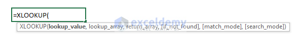
The XLOOKUP function searches a range or an array for a match and returns the corresponding item from the second range or array. By default, an exact match is used. The generic formula of this function is as follows:
=XLOOKUP(lookup_value, lookup_array, return_array, [if_not_found], [match_mode], [search_mode])
VLOOKUP Function
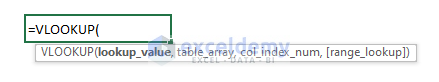
The VLOOKUP function looks for a value in the leftmost column of a table and then returns a value in the same row from a specified column. By default, the table must be sorted in ascending order. The generic formula of this function looks like this:
=VLOOKUP(lookup_value, table_array, col_index_num, [range_lookup])
Arguments of the XLOOKUP Function
| Argument | Required/Optional | Explanation |
|---|---|---|
| lookup_value | Required | The specified value that is to be searched for in the data table. |
| lookup_array | Required | A range of cells or an array where the lookup value will be searched for. |
| return_array | Required | The second range of cells or an array from where the output data will be extracted. |
| [if_not_found] | Optional | Customized message in a text format, if the lookup value is not found. |
| [match_mode] | Optional | It defines if the function will look for an exact match based on specified criteria or a wildcard character match. |
| [search_mode] | Optional | It defines the search order (In ascending or descending, from last to first or first to last). |
Arguments of the VLOOKUP Function
| Argument | Required/Optional | Explanation |
|---|---|---|
| lookup_value | Required | The specified value that is to be searched for in the data table. |
| table_array | Required | A range of cells or an array where the lookup value will be searched for. |
| col_index_num | Required | The index number of the column in the specified array, where the return value is present. |
| [range_lookup] | Optional | Defines the exact or approximate match. |
XLOOKUP vs. VLOOKUP Function in Excel: 5 Comparative Examples
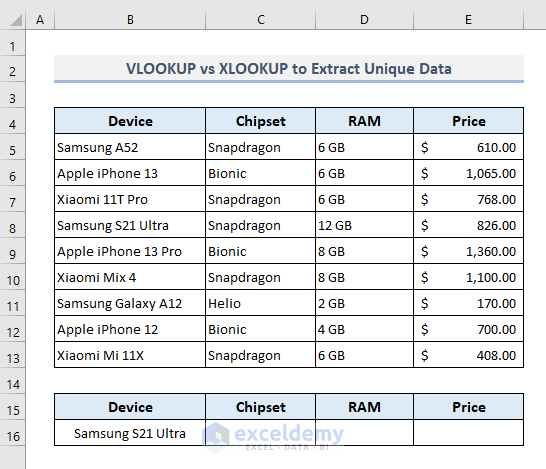
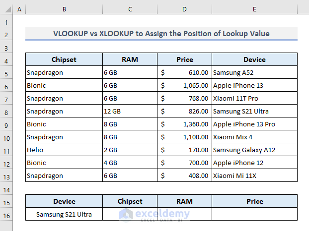
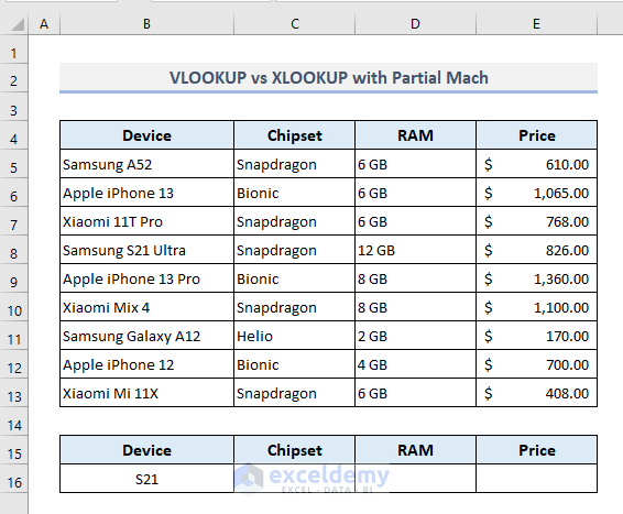
Example 1 – XLOOKUP and VLOOKUP to Lookup Unique Value and Extract Data
We’re going to extract the specifications of the Samsung S21 Ultra from the data table.
We’re going to apply the VLOOKUP function first. In the output Cell C16, the required formula will be:
=VLOOKUP(B16,B5:E13,{2,3,4},FALSE)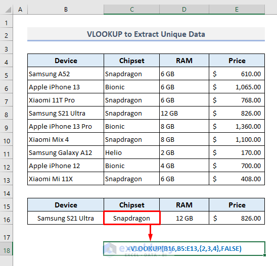
If we use the XLOOKUP function instead of the VLOOKUP function, the output Cell C16 needs the following formula:
=XLOOKUP(B16,B5:B13,C5:E13,,0)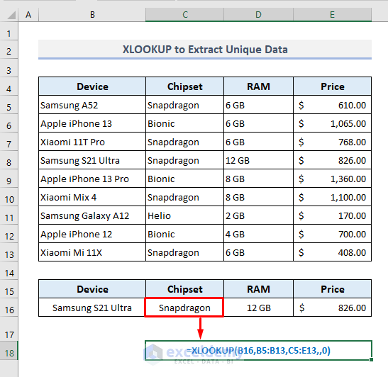
The basic difference between using these two functions is the VLOOKUP function has extracted multiple values based on the specified column numbers in an array, while the XLOOKUP function has returned a similar output by taking a range of cells containing the specifications as a return array argument.
Read More: INDEX MATCH vs VLOOKUP Function
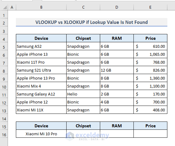
Example 2 – VLOOKUP Is Unable to Show a Message If the Lookup Value Is Not Found
We’re going to find the specifications of the Xiaomi Mi 10 Pro in the following table.
As the lookup value is lying in Cell B16, the required formula with the VLOOKUP function in the output Cell C16 will be:
=VLOOKUP(B16,B5:E13,{2,3,4},FALSE)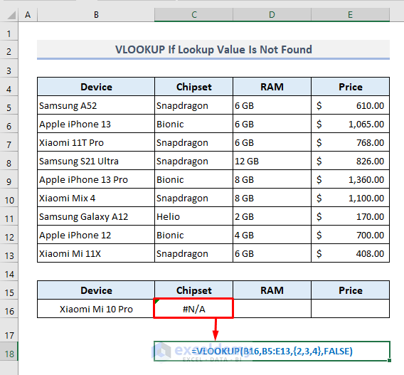
If you customize a message with the XLOOKUP function if the lookup value is not found, the required formula in Cell C16 could look like this:
=XLOOKUP(B16,B5:B13,C5:E13,"Not Found",0)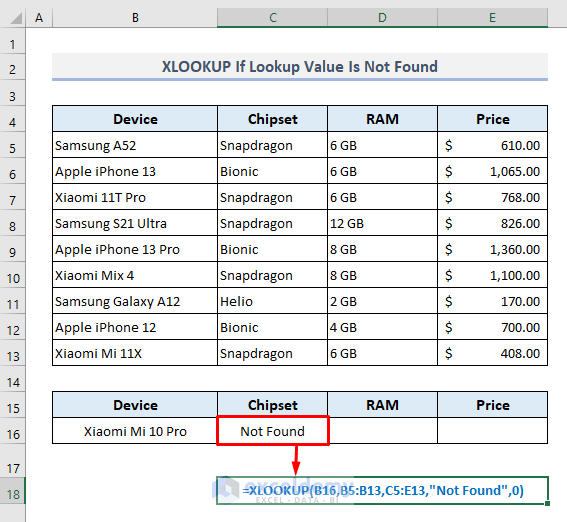
If you want to display a customized message with the VLOOKUP function, you have to combine the IF function with the VLOOKUP function.
Read More: Excel LOOKUP vs VLOOKUP
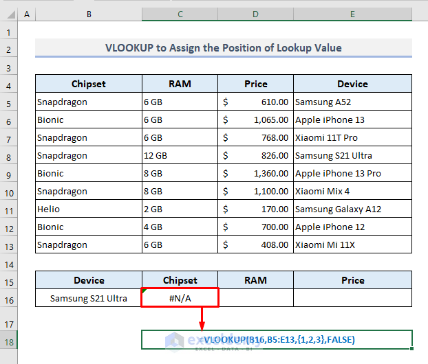
Example 3 – VLOOKUP Searches for the Value in the Leftmost Column Only
We’ll find out the output the function will return if we look for a value in the rightmost column in the table.
The required function in Cell C16 will be:
=VLOOKUP(B16,B5:E13,{1,2,3},FALSE)After pressing Enter, you’ll find a #N/A error as the return output. So, it’s now understood that while using the VLOOKUP function, you have to look for a value only in the leftmost column, otherwise, the function will not display the expected result.
To extract the available data from the table for the specified device present in Cell B16, the XLOOKUP function will be:
=XLOOKUP(B16,E5:E13,B5:D13,,0)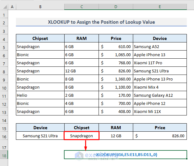
Read More:Excel VLOOKUP to Find Last Value in Column
Example 4 – Extract Data Based on the Last Occurrence with XLOOKUP Only
We can find out which smartphone device in Column B is the last one that uses the Bionic chipset.
The required formula with the XLOOKUP function in Cell C16 should be:
=XLOOKUP(B16,C5:C13,B5:B13,,0,-1)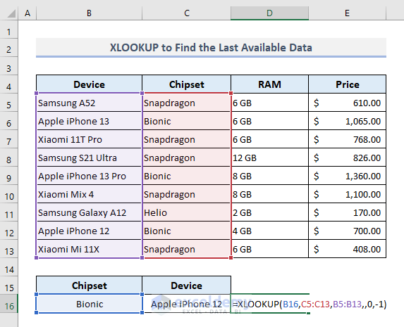
In the function, we have used the [search_mode] argument where ‘-1’ implies that the function will look for the value from the last to the first. If you opt to choose ‘1’ here, then the function will look out from the first to the last.
The VLOOKUP function itself is not able to extract the data based on the last occurrence in a table. It might have to be combined with some other functions to look up the value from the last in the data table.
Example 5 – XLOOKUP Takes an Optional Argument to Use Wildcard Characters
We’re going to find out the available specifications by searching for the model number ‘S21’ of a smartphone device.
With the Wildcard Characters as well as Ampersand (&) operators, the VLOOKUP function in the output Cell C16 will look like this:
=VLOOKUP("*"&B16&"*",B5:E13,{2,3,4},FALSE)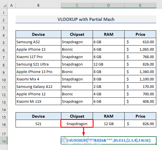
While using the XLOOKUP function, we have to activate the [match_mode] argument and define it with ‘2’ to denote the Wildcard Characters matches. The required function in Cell C16 will look like this:
=XLOOKUP("*"&B16&"*",B5:B13,C5:E13,,2)
Why Is XLOOKUP Better Than VLOOKUP?
- In the XLOOKUP function, you have to specify a range of cells or an array as the return array which is way too easy to denote from the data table. In the VLOOKUP function, while extracting multiple values from the table, you have to manually specify the index numbers of the columns in an array where the return values are present, and sometimes it’s quite tricky to find the index numbers from a large dataset.
- The XLOOKUP function is handier when you have to show a customized message if the lookup value is not found. The VLOOKUP function cannot show any customized message itself.
- The VLOOKUP function looks for a value in the leftmost column in a table whereas the XLOOKUP function looks for a value in any column in the given data table.
- With the VLOOKUP function, you have to specify the entire table array where the lookup value and return value(s) are present. In the XLOOKUP function, you have to define the lookup array and the return array separately.
- The XLOOKUP function searches a lookup value from the bottom to top in the given dataset whereas, the VLOOKUP needs other functions to extract data based on the last occurrence in the table.
- The XLOOKUP function allows you to go for a binary search, the VLOOKUP function doesn’t come up with such a criterion.
- With the VLOOKUP function, you can use the approximate match to return the next smaller value only. But with the XLOOKUP function, you’ll be able to return any of the next smaller or next larger values from the table.
Limitations of XLOOKUP in Excel
There might be only one specific drawback with the XLOOKUP function and that is its availability in Microsoft Excel 365. The XLOOKUP function is not compatible with older versions. However, the VLOOKUP function is available to use in any version of Excel.
Download the Practice Workbook
Related Articles
- Combining SUMPRODUCT and VLOOKUP Functions in Excel
- How to Use VLOOKUP with COUNTIF
- How to Combine SUMIF and VLOOKUP in Excel
- Use VLOOKUP to Sum Multiple Rows in Excel
- How to Use Nested VLOOKUP in Excel
- IF and VLOOKUP Nested Function in Excel
- How to Use IF ISNA Function with VLOOKUP in Excel
- How to VLOOKUP and SUM Across Multiple Sheets in Excel
- How to Use IFERROR with VLOOKUP in Excel
- VLOOKUP with IF Condition in Excel
<< Go Back to Excel VLOOKUP Function | Excel Functions | Learn Excel
Get FREE Advanced Excel Exercises with Solutions!

2. VLOOKUP is Unable to Show Message If Lookup Value Is Not Found
You can use the :=IFERROR(VLOOKUP(B16,B5:E13,{2,3,4},FALSE),”Not Found”)
OR =IF(ISERROR(VLOOKUP(B16,B5:E13,{2,3,4},FALSE))=TRUE,”Not Found”,VLOOKUP(B16,B5:E13,{2,3,4},FALSE))
4. Extract Data Based on the Last Occurrence with XLOOKUP Only
Use auxiliary columns ,=C5&COUNTIF(C5:$C$5,C5),
And then pull down.
objectives :Bionic3
=VLOOKUP(B18,CHOOSE({1,2},F5:F13,B5:B13),2,0)
Hello Yaojm,
Thanks for your suggestions. Here we focused on the comparison/difference of VLOOKUP and XLOOKUPp that’s why we didn’t improvised the use of VLOOKUP.
Regards
ExcelDemy
How do we use V-lookup or X-Lookup functions to calculate very fastly, GPA & CGPA of group of students with different scores in different courses from year to year ?
Hi, Icide. M. O.
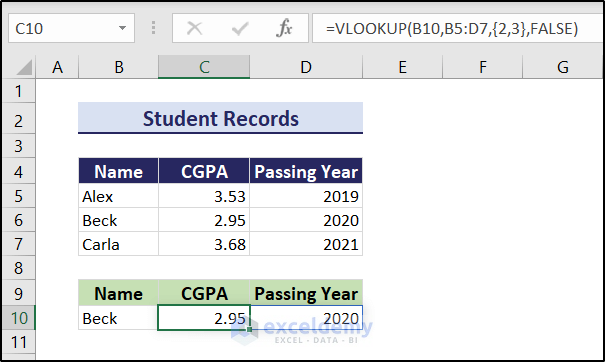
VLOOKUP or XLOOKUP is specifically for finding a value from a table/range. If you have the CGPA already calculated, you can use these functions to find it like this.
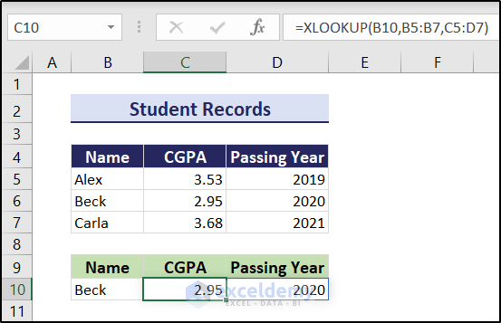
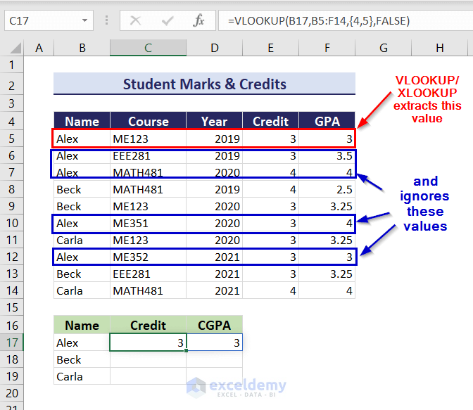
Similarly, you can use the XLOOKUP function too.
Assuming you don’t have the CGPAs already calculated, you want to do that from grades within Excel, you need all the grades for a certain person. If you have multiple values matching in a range, the VLOOKUP/XLOOKUP only returns the first match.
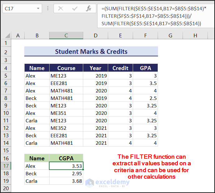
However, there are other workarounds for this. For example, the FILTER function can extract all the matching values. You can use them to your calculation’s advantage after that.
Here, I have used the Σfixi/Σfi formula to calculate the CGPA assuming it has a credit system. I have also used the absolute referencing as you have mentioned replicating the formula for a group of students. Hopefully, this answered your question.
If you are still struggling with your particular dataset, feel free to let me know. I will try to get back to you.
Regards
Niloy, Team Exceldemy