If you are looking for ways to use a combination of the INDIRECT and VLOOKUP functions in Excel, then you will find this article useful. The INDIRECT function in Excel helps the users lock the specified cell in a formula. Therefore, without changing the formula itself, we can modify cell references within a formula. Sometimes while working with multiple databases we need to perform dynamic VLOOKUP in those databases for values. We can do this easily with the combination of the INDIRECT and the VLOOKUP function. In this article, we will learn how to perform the INDIRECT VLOOKUP formula.
Quick View
Let’s take a quick view of today’s task.
Use of VLOOKUP Function with INDIRECT Function in Excel: 3 Examples
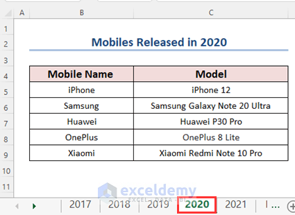
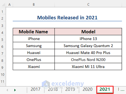
Here, we have some lists of models of different mobile companies for 2017, 2018, 2019, 2020, and 2021 in different sheets. Using a combination of these functions we will extract our desired values from these sheets in a new sheet.
For creating this article, we have used the Microsoft Excel 365 version. However, you can use any other version at your convenience.
Example-1: Extracting Values from Different Sheets by Using INDIRECT and VLOOKUP Functions
Here is a scenario for using the combination of these functions. Consider you have an assignment where you are given some mobile phone name and their model data from 2017-2021. Now you have to assemble those names and their model systematically in a new worksheet. the INDIRECT function and VLOOKUP formula can easily do this. Let’s learn!
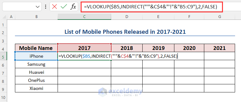
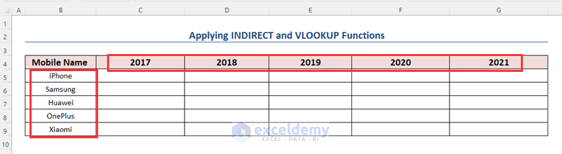
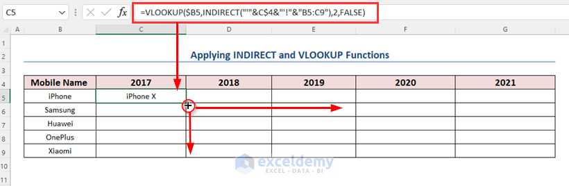
We created a table in a new worksheet. This table contains the “Mobile Name” column and the associated years “2017”, “2018”, “2019”, “2020”, and “2021” columns. We need to retrieve the model from these years from their respective sheets for the given “Mobile Name”.
Steps:
- Now we will apply the “INDIRECT VLOOKUP” formula.
The generic formula is,
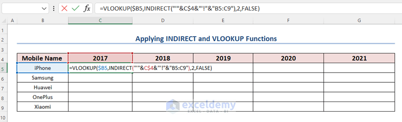
=VLOOKUP(lookup_value, INDIRECT(“Table_Array”), col_index,0)- Now insert the values into the formula in cell C5 and the final formula is
=VLOOKUP($B5,INDIRECT("'"&C$4&"'!"&"B5:C9"),2,FALSE)Formula Breakdown
- Lookup_value is $B4
- Table_array is created using this function INDIRECT(“‘”&C$3&”‘!”&”B4:C8”). The mixed reference C$3 refers to the column heading (2017) which matches the worksheet names. The “Concatenation Operator (&)” is used to join the single quote character(“&C$3&”) to either side. To create a specific worksheet reference, the “Exclamation Point (!)” is joined on the right side of the formula. The output of this concatenation is a “Text” which will be used in the “INDIRECT” function as a reference.
- Column_index_number is “2”.
- We want the EXACT match (FALSE).
- Press ENTER and drag down and to the right the Fill Handle tool.
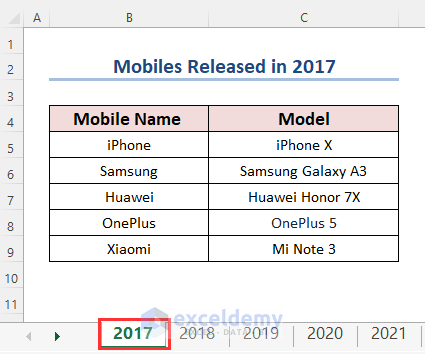
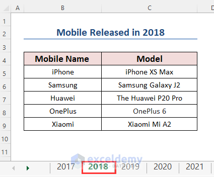
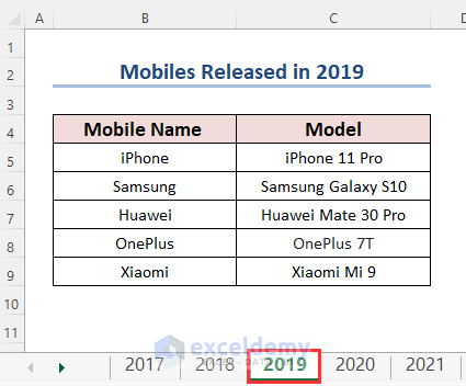
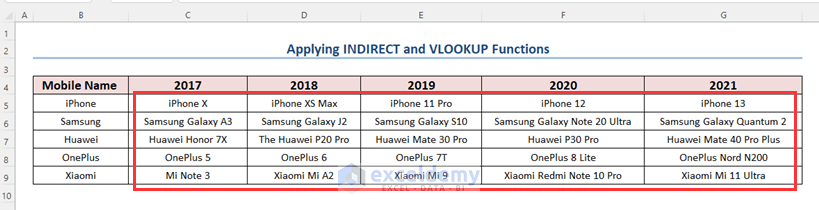
In this way, you will be able to extract all of the models of different mobile companies respective to their years.
Read More:How to Use VLOOKUP Function with Exact Match in Excel
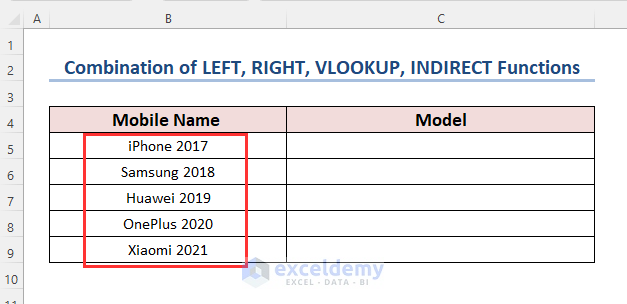
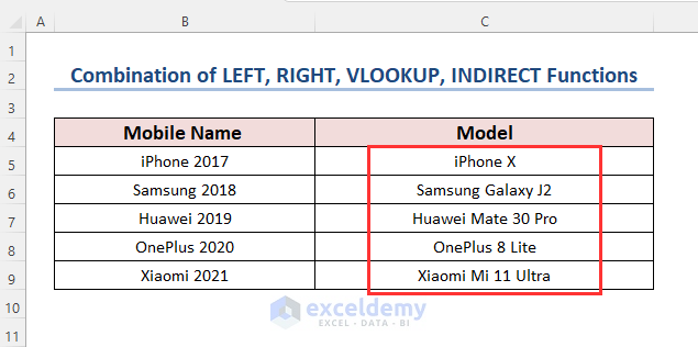
Example-2: Getting Values from Different Sheets by Using INDIRECT, VLOOKUP, LEFT, and RIGHT Functions
In this section, we have different names of mobile companies joined together with their years. Our task is to search for the respective model names of this mobile company for that particular year. To do this, we will use a combination of the LEFT, RIGHT, FIND, INDIRECT, and VLOOKUP functions.
Steps:
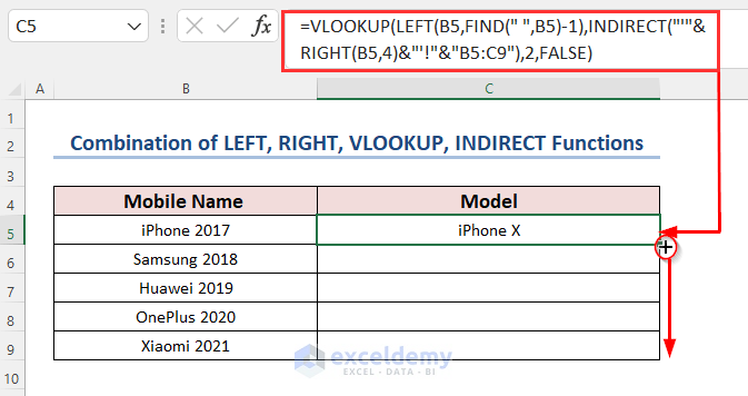
- Apply the following formula in cell C5.
=VLOOKUP(LEFT(B5, FIND(" ", B5)-1), INDIRECT("'"&RIGHT(B5,4)&"'!"&"B5:C9"),2, FALSE)Formula Breakdown
- FIND(” “, B5) → becomes
- FIND(” “, “iPhone 2017”) → finds the position of space in this text string
- Output → 7
- FIND(” “, “iPhone 2017”) → finds the position of space in this text string
- FIND(” “, B5)-1 → becomes
- 7-1 → 6
- LEFT(B5, FIND(” “, B5)-1) → becomes
- LEFT(“iPhone 2017”,6) → extracts the first 6 characters from this text string
- Output → “iPhone”
- LEFT(“iPhone 2017”,6) → extracts the first 6 characters from this text string
- RIGHT(B5,4) → becomes
- RIGHT(“iPhone 2017”,4) → extracts the last 4 characters from the right side of this text string.
- Output → 2017
- RIGHT(“iPhone 2017”,4) → extracts the last 4 characters from the right side of this text string.
- INDIRECT(“‘”&RIGHT(B5,4)&”‘!”&”B5:C9”) → becomes
- INDIRECT(“‘”&“2017”&”‘!”&”B5:C9”)
- Output → ‘2017’!B5:C9
- INDIRECT(“‘”&“2017”&”‘!”&”B5:C9”)
- VLOOKUP(LEFT(B5,FIND(” “,B5)-1),INDIRECT(“‘”&RIGHT(B5,4)&”‘!”&”B5:C9”),2,FALSE) → becomes
- VLOOKUP(“iPhone”, ‘2017’!B5:C9,2, FALSE) → extracts the model name for 2017 of this company
- Output → iPhone X
- VLOOKUP(“iPhone”, ‘2017’!B5:C9,2, FALSE) → extracts the model name for 2017 of this company
- Drag down and to the right the Fill Handle.
Eventually, you will have the following models in the Model column.
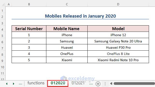
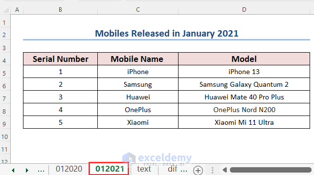
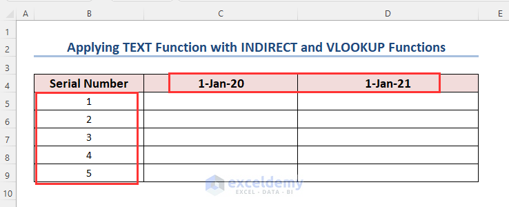
Example-3: Combination of INDIRECT, VLOOKUP, and TEXT Functions
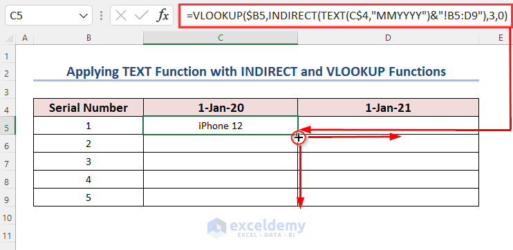
Here, we have the following two datasets of mobile models for 2020, and 2021. And the name of these sheets is- 012020, and 012021, representing January month of these years.
In a new sheet, we have created the following table. In the Serial Number column, we have some numbers on the basis of which we will look for the values in other sheets. And the other columns have dates as their headers with the help of which we will find out our sheets.
Steps:
- Apply the following formula in cell C5.
=VLOOKUP($B5, INDIRECT(TEXT(C$4, "MMYYYY")&"!B5:D9"),3,0)Formula Breakdown
- TEXT(C$4, “MMYYYY”) → becomes
- TEXT(43831, “MMYYYY”) → The TEXT function will format the date value as MMYYYY.
- Output → 012020
- TEXT(43831, “MMYYYY”) → The TEXT function will format the date value as MMYYYY.
- INDIRECT(TEXT(C$4, “MMYYYY”)&”!B5:D9″) → becomes
- INDIRECT(“012020″&”!B5:D9″)
- Output → ‘012020’!B5:D9
- INDIRECT(“012020″&”!B5:D9″)
- VLOOKUP($B5, INDIRECT(TEXT(C$4, “MMYYYY”)&”!B5:D9″),3,0) → becomes
- VLOOKUP(1, ‘012020’!B5:D9,3,0)
- Output → iPhone 12
- VLOOKUP(1, ‘012020’!B5:D9,3,0)
- Drag down and to the right the Fill Handle.
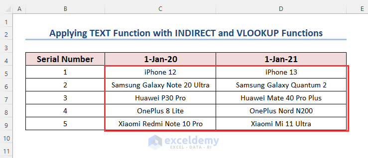
Ultimately, you will get the following results.
Read More:VLOOKUP Example Between Two Sheets in Excel
How to Use INDIRECT and VLOOKUP Functions for Different Workbooks in Excel
In the following figures, we have 2 separate workbooks; 2020.xlsx, and 2021.xlsx, with their worksheets; 2020, and 2021. From these workbooks, we will extract our needed values into a new workbook.
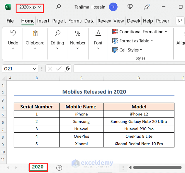
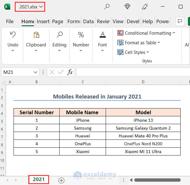
To extract the model names, we have created the following dataset in a new workbook.
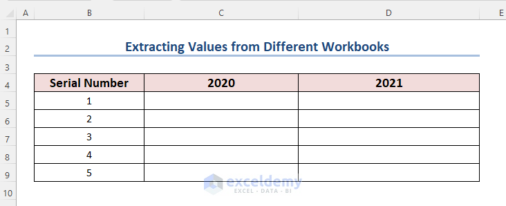
Steps:
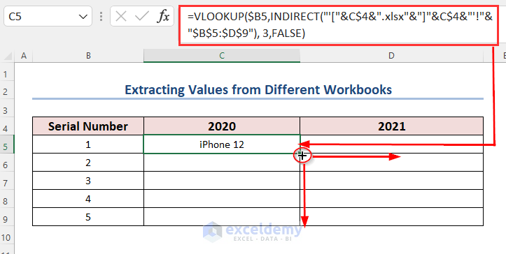
- Enter the following formula in cell C5.
=VLOOKUP($B5,INDIRECT("'["&C$4&".xlsx"&"]"&C$4&"'!"&"$B$5:$D$9"), 3,FALSE)Formula Breakdown
- “‘[“&C$4&”.xlsx”&”]” → becomes
- “‘[“&2020&”.xlsx”&”]” → The Ampersand operator will join these strings
- Output → “‘[2020.xlsx]”
- “‘[“&2020&”.xlsx”&”]” → The Ampersand operator will join these strings
- INDIRECT(“‘[“&C$4&”.xlsx”&”]”&C$4&”‘!”&”$B$5:$D$9″) → becomes
- INDIRECT(“‘[2020.xlsx]”&2020&”‘!”&”$B$5:$D$9”)
- Output → ‘2020.xlsx’!$B$5:$D$9
- INDIRECT(“‘[2020.xlsx]”&2020&”‘!”&”$B$5:$D$9”)
- VLOOKUP($B5,INDIRECT(“‘[“&C$4&”.xlsx”&”]”&C$4&”‘!”&”$B$5:$D$9″), 3,FALSE) → becomes
- VLOOKUP(1,’2020.xlsx’!$B$5:$D$9, 3,FALSE)
- Output → iPhone 12
- VLOOKUP(1,’2020.xlsx’!$B$5:$D$9, 3,FALSE)
- Drag down and to the right the Fill Handle.
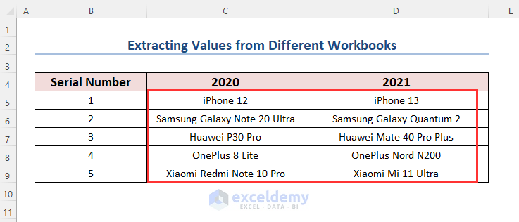
Eventually, we extracted the following mobile models from different workbooks.
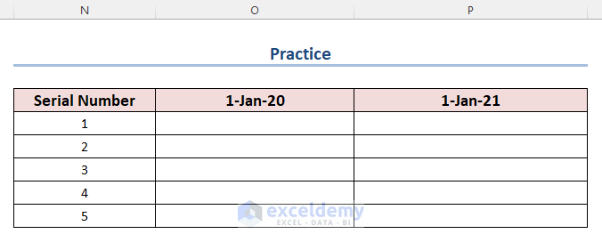
Practice Section
To practice by yourself, we have created a Practice section on the right side of each sheet.
Things to Remember
⏩For the INDIRECT function, if ref_text is not a valid cell reference, the function will return the #REF! error value.
⏩The VLOOKUP function always searches for lookup values from the leftmost top column to the right. This function “Never” searches for the data on the left.
⏩When you select your “Lookup_value” you have to use the absolute cell references ($) to block the array.
Download Practice Workbook
Conclusion
The powerful combo “INDIRECT VLOOKUP” is discussed using an example in this article. We hope this article proves useful to you. If you have any thoughts regarding this article please do share them in our comment section.
Further Readings
- Combining SUMPRODUCT and VLOOKUP Functions in Excel
- How to Use VLOOKUP with COUNTIF
- How to Combine SUMIF and VLOOKUP in Excel
- Use VLOOKUP to Sum Multiple Rows in Excel
- INDEX MATCH vs VLOOKUP Function
- Excel LOOKUP vs VLOOKUP
- XLOOKUP vs VLOOKUP in Excel
- How to Use Nested VLOOKUP in Excel
- IF and VLOOKUP Nested Function in Excel
- How to Use IF ISNA Function with VLOOKUP in Excel
- How to VLOOKUP and SUM Across Multiple Sheets in Excel
- How to Use IFERROR with VLOOKUP in Excel
- VLOOKUP with IF Condition in Excel
<< Go Back to VLOOKUP a Range | Excel VLOOKUP Function | Excel Functions | Learn Excel
Get FREE Advanced Excel Exercises with Solutions!
