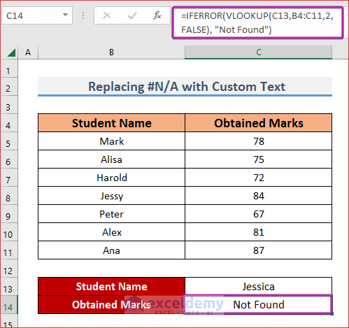
Method 1 – Replace #N/A with Custom Text
Search for a student whose name isn’t in the list, you want to show custom text such as “Not found”. Enter the following formula in cell C14 and press ENTER to do the task.
C13 = Lookup value, which will be searched in the list Type any student name from your list in cell C13; you will get his/her obtained marks in cell C14. Type any student name that isn’t on your list in cell C13; the C14 cell will show your custom text Not Found. Keep the cell empty when the searched name isn’t in your list, type the following formula in cell C13, C13 = Lookup value which will be searched in the list Type any student name from your list in cell C13; you will get his/her obtained marks in cell C14. Type any name that isn’t in the dataset, the cell C14 will remain empty. You have two lists in your dataset. You want to find the obtained marks for any student from both lists. Type the following formula in cell C13 and press ENTER. C13 = Lookup value, which will be searched in the list Type any of the names from any of your lists, in cell C13, you will get the obtained marks of that person in cell C14. You have contact numbers of different branches of your company in your dataset. You want to show a contact number if anyone searches for any of the branches, even if the branch name isn’t on your list. If the branch name isn’t on the list, you want to show the contact number of the Head office. Type the following formula in any empty cell and press ENTER. C13 = Lookup value, which will be searched in the list Type any branch name in cell C10 that isn’t in the list; you will get the contact number of the head office in the cell where you typed the formula. In Excel 2013 or in any older version the IFERROR function isn’t available, but you can do the same task by using the IF function and the ISNA function along with the VLOOKUP function. Type the following formula in cell C14 and press ENTER C13 = Lookup value, which will be searched in the list Type any student name from your list in cell C13; you will get his/her obtained marks in cell C14. Type any student name that isn’t in your list in cell C13; Cell C14 will show your custom text Not Found. Download Practice Workbook Download this practice workbook to exercise while you are reading this article. << Go Back to VLOOKUP with IF Condition | Excel VLOOKUP Function | Excel Functions | Learn Excel=IFERROR(VLOOKUP(C13,B4:C11,2,FALSE), "Not Found")
B4:C11 = Lookup range that is your dataset
2 = Lookup column that is the column of Obtained Marks
FALSE means the function will look for an exact match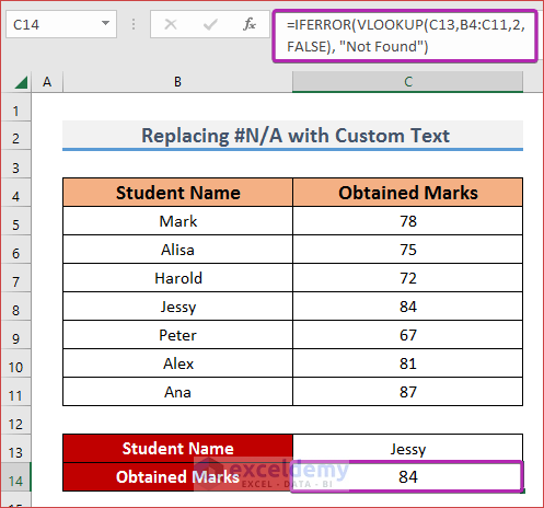
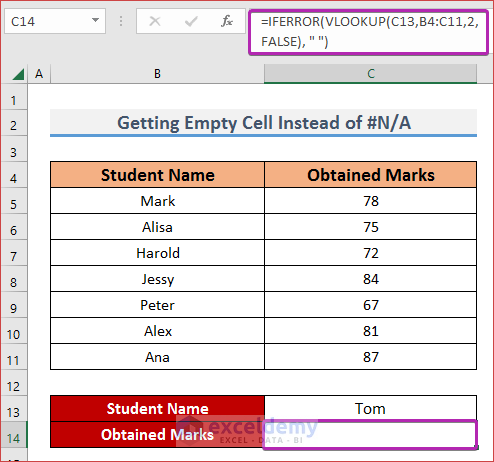
Method 2 – Get Empty Cell Instead of #N/A
=IFERROR(VLOOKUP(C13,B4:C11,2,FALSE), " ")
B4:C11 = Lookup range that is your dataset
2 = Lookup column that is the column of Obtained Marks
FALSE means the function will look for an exact match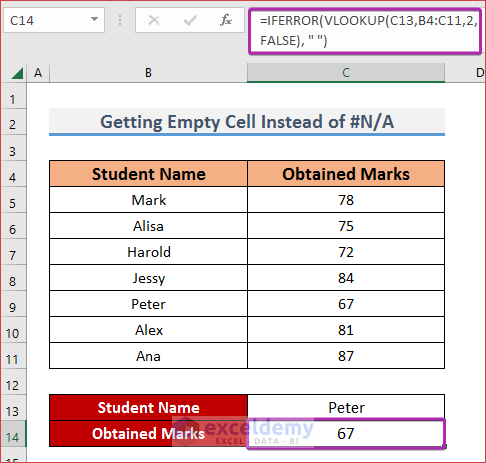
Method 3 – IFERROR with VLOOKUP for Split Dataset
=IFERROR(VLOOKUP(C13,B4:C11,2,FALSE),VLOOKUP(C13,B14:C20,2,FALSE))
B4:C11 =1st lookup range that is the 1st list of the dataset
B14:C20 = = 2nd lookup range that is the 2nd list of the dataset
2 = Lookup column that is the column of Obtained Marks
FALSE means the function will look for an exact match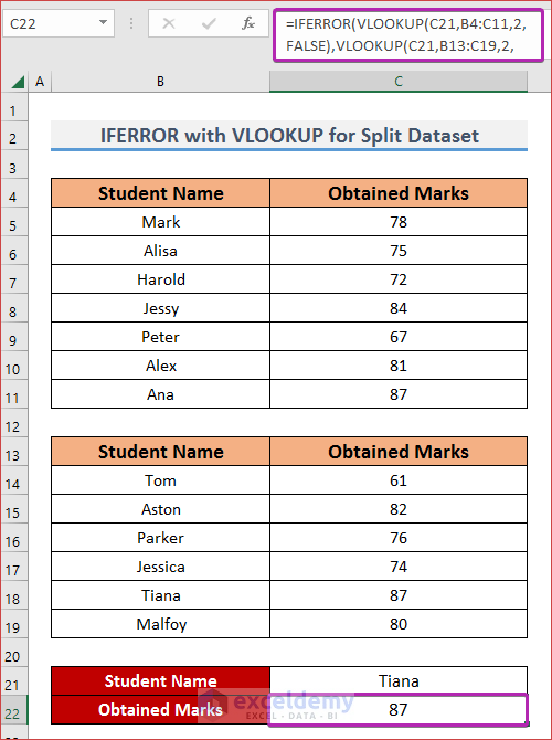
Method 4 – IFERROR with VLOOKUP to Return Output Every Time
=IFERROR(VLOOKUP(C13,B4:C8,2,FALSE),VLOOKUP("Head office",B4:C8,2,FALSE))
B4:C11 = Lookup range that is your dataset
2 = Lookup column that is the column of Contact Number
FALSE means the function will look for an exact match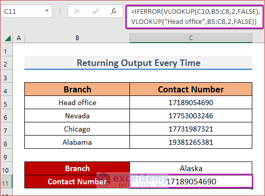
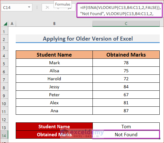
Method 5 – Apply VLOOKUP in Older Version of Excel
=IF(ISNA(VLOOKUP(C13,B4:C11,2,FALSE)), "Not Found", VLOOKUP(C13,B4:C11,2,FALSE))
B4:C11 = Lookup range that is your dataset
2 = Lookup column that is the column of Contact Number
FALSE means the function will look for an exact match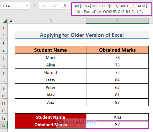
Further Readings

