Microsoft Excel is a powerful tool for organizing and analyzing data, but sometimes our data isn’t always clean and error-free. That’s where the IFERROR function comes in handy. The IFERROR function allows us to specify what should happen when an error occurs in a formula. In this article, I am going to explain 2 smart ways on the topic of how to use multiple IFERROR statements in Excel. I hope it will be very helpful for you if you are looking for an efficient way to do so.
How to Use Multiple IFERROR Statements in Excel: 2 Smart Ways
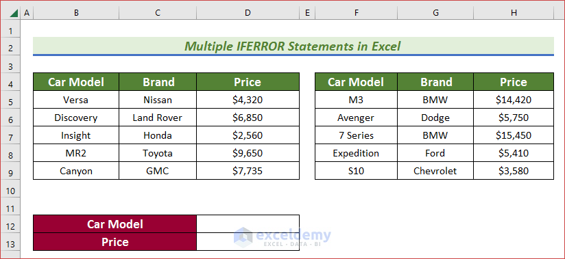
In terms of explaining the use of multiple IFERROR statements, I am going to use the following dataset where I have arranged cars’ descriptions in the Car Model, Brand, and Price columns. I have also combined the VLOOKUP function and the IF function with IFERROR. Let’s dive into detail.
1. Multiple IFERROR Statements with VLOOKUP
In the case of searching for a certain result in different ranges, we can use multiple IFERROR statements combined with VLOOKUP. The process is discussed in detail in the following section.
Steps:
- First of all, set a value in a cell to look for. Here, I want to find the price of a certain car. So, I assigned the car name (i.e. Avenger) in the Car Model section.
- Then, apply the following formula in your preferred location and press ENTER to have your desired output.
=IFERROR(VLOOKUP(D12,B5:D9,3,FALSE),IFERROR(VLOOKUP(D12,F5:H9,3,FALSE),"Not Found"))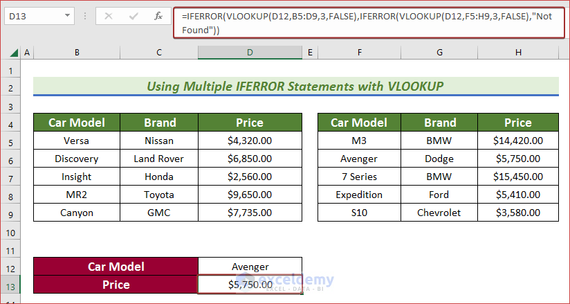
- If the search value does not appear in that range, it will return the defined output according to the value set in the formula. In my case, I have set Not Found as a return if the search value does not appear in that range.

2. IF Function with Multiple IFERROR Statements
We can check a certain value whether belongs to the defined ranges with a combination of multiple IFERROR statements and IF function. It is not a big deal. You will know it after learning the following section.
Steps:
- Input a value in a cell to check whether it belongs to the defined ranges.
- Next, insert the following formula with a returned value when it belongs to that range or not. Here, If the search value belongs to the range B5:D9 or F5:H9, it will return Exist in the Table.
=IF(IFERROR(VLOOKUP(D12,B5:D9,3,FALSE),IFERROR(VLOOKUP(D12,F5:H9,3,FALSE),"Not Found"))="Not Found","Need to Add","Exist in the Table")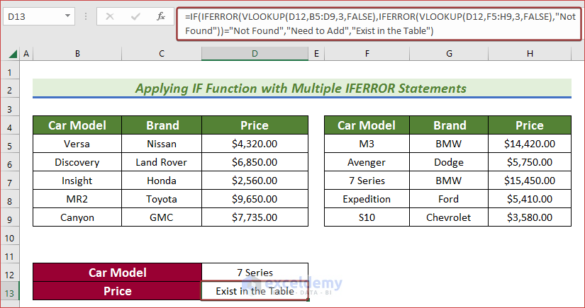
- Otherwise, it will return Need to Add.

How to Combine SUM and IFERROR Functions in Array in Excel
In terms of applying IFERROR in arrays, we can also combine the SUM function with IFERROR to have a summation. To find the total number of products sold, you need to divide the Total Price of each product by the Unit Price and then add them. We can lessen your workload just by applying the following formula.
=SUM(IFERROR($C$5:$C$9/$D$5:$D$9,0))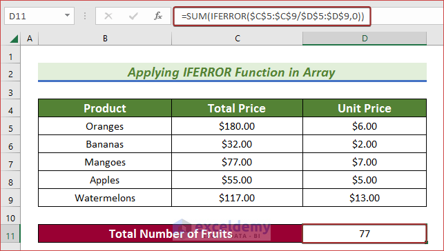
Download Practice Workbook
Download this practice workbook to exercise while you are reading this article.
Conclusion
At the end of this article, I like to add that I have tried to explain 2 smart ways on the topic of how to use multiple IFERROR statements in Excel. It will be a great pleasure for me if this article helps any Excel user even a little. For any further queries, comment below. You can visit our site for more articles about using Excel.
Related Articles
- Excel ISERROR vs IFERROR Functions
- How to Use Conditional Formatting with IFERROR in Excel
- Excel IFERROR Function to Return Blank Instead of 0
<< Go Back to Excel IFERROR Function | Excel Functions | Learn Excel
Get FREE Advanced Excel Exercises with Solutions!
