Looking for differences between Excel ISERROR and IFERROR functions? Then, this is the right place for you. Sometimes, we may find different kinds of errors while using a formula. In those cases, you may use the ISERROR or IFERROR function to resolve the issue. However, these functions have different approaches to solving errors and returning results. Here, you will find 2 different examples of using ISERROR vs IFERROR functions in Excel.
Introduction to Excel ISERROR Function

- Function Objective:
The ISERROR function is used to check if the value of a cell shows an error or not.
- Syntax:
=ISERROR(value)
- Arguments Explanation:
| ARGUMENT | REQUIRED/OPTIONAL | EXPLANATION |
| value | Required | Insert value to check if there is any error |
- Return Parameter:
Returns TRUE there is any error, otherwise returns FALSE.
- Version:
This function is available for Excel 2003 through 2021 and Excel 365.
Introduction to Excel IFERROR Function
- Function Objective:
The IFERROR function is used to check if there is any error. It can return the usual result for no error and returns an alternate result if there is any.
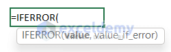
- Syntax:
=IFERROR(value,value_if_error)
- Arguments Explanation:
| ARGUMENT | REQUIRED/OPTIONAL | EXPLANATION |
| value | Required | The value, reference, or formula to check for an error. |
| value_if_error | Required | The result you want if error occurs |
- Return Parameter:
Returns value that we have inserted for both errors and without any error.
- Version:
This function is available for Excel 2010, Excel 2013, Excel 2016, Excel 2019, Excel 2021, and Excel 365.
Excel ISERROR vs IFERROR Functions: 2 Suitable Examples
The IFERROR function is used to check if there is any error or not. On the other hand, the IFERROR function can be used to avoid errors and return the desired result if there is any error. Here, we will show you 2 examples to show the difference between these two functions.
1. Remove #DIV/0! Error Using Excel ISERROR and IFERROR Functions
In the first example, we will show you how to remove #DIV/0! Error using both ISERROR and IFERROR functions.
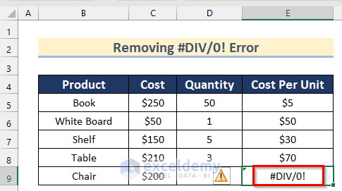
Suppose we have a dataset containing information on some Products, their Cost, and Quantity. Now, we will show you how you can find out the Cost Per Unit of these products and handle #DIV/0! Error.

Steps:
- Firstly, select Cell E5 and insert the following formula.
=C5/D5
- Then, press Enter and drag down the Fill Handle tool to AutoFill the formula for the rest of the cells.

Here, in the formula, we divided the value of Cell C5 by the value of Cell D5 to get the Cost per Unit of Books.
- Thus, you will find all the values of Cost Per Unit for all the products.
- Here, you can see that #DIV/0! error has occurred in Cell E9 as there is no value in Cell D9.
- However, to check this error you can use the ISERROR function.
- Next, to do that, insert the following formula in Cell F5 and press Enter.
=ISERROR(E5)
- After that, drag down the Fill Handle tool to AutoFill the formula for the rest of the cells.
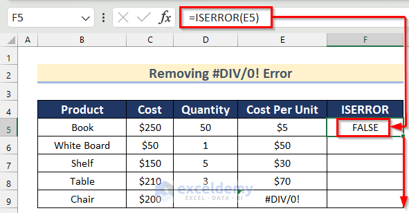
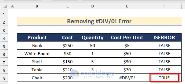
In the ISERROR function, we insert Cell E5 as value to check for an error.
- Now, you can see that Cell F9 returns TRUE as there is an error in Cell E9.
- On the other hand, using the IFERROR function you can remove the error and return the desired value.
- Firstly, select Cell G5 and insert the following formula.
=IFERROR(E5,"Not Determined")
- Then, drag down the Fill Handle tool up to Cell G9.
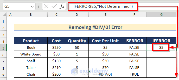
In the IFERROR function, we inserted Cell E5 as value and “Not Determined” as value_if_error.
- Thus, you can remove an error using the IFERROR function.

2. Combine Excel VLOOKUP Function with ISERROR VS IFERROR Functions to Ignore Error
In this example, we will show you how to combine the VLOOKUP function with ISERROR vs IFERROR functions in Excel.
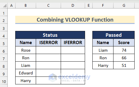
Here, we have a dataset containing the Name and Score of students who have passed. Now, using this dataset we will update the Status of some students if they have passed or failed and show you the difference between using the ISERROR and IFERROR functions.
Steps:
- In the beginning, insert the following formula in Cell C6.
=IF(ISERROR(VLOOKUP(B6,$F$6:$G$8,2,FALSE)),"Failed",VLOOKUP(B6,$F$6:$G$8,2,FALSE))
- Then, press Enter and drag down the Fill Handle tool for the rest of the cells.

- Thus, you will get the score for students who have passed and the Status also gets updated for those who have failed.

🔎 How Does the Formula Work?
- Firstly, we used the VLOOKUP function to check if Cell B6 is in cell range F6:G8 or not.
- Then, we used the ISERROR function to check for any error.
- Lastly, we used the IF function to return the “Failed” if there is an error or to return the Score if the student passed.
- On the contrary, to use the IFERROR function in this case, insert the following formula in Cell D6 and press Enter.
=IFERROR(VLOOKUP(B6,$F$6:$G$8,2,FALSE),"Failed")
- After that, use the Fill Handle tool to autofill the formula for the rest of the cells.
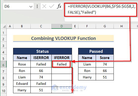
- Similarly, you will get the score for students who have passed and the Status also gets updated for those who have failed.

🔎 How Does the Formula Work?
- Firstly, we used the VLOOKUP function to look up the value of Cell B6 from cell range F6:G8.
- Then, we used the IFERROR function to return the Score of that student if he/she passed or else to return “Failed”.
Read More: How to Use IFERROR with VLOOKUP in Excel
Differences Between ISERROR and IFERROR Functions in Excel
Though both ISERROR and IFERROR functions deal with errors, there are some clear differences between them.
|
ISERROR Function |
IFERROR Function |
|
|
|
|
|
|
Practice Section
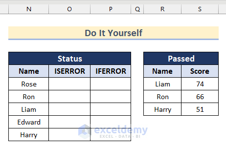
In this section, we are giving you the dataset to practice on your own and learn to use these methods.
Download Practice Workbook
You are welcome to download the practice workbook from the link below.
Conclusion
So, in this article, you will find 2 examples of using ISERROR vs IFERROR functions in Excel. Use any of these ways to accomplish the result in this regard. Hope you find this article helpful and informative. Feel free to comment if something seems difficult to understand. Additionally, let us know any other approaches which we might have missed here. Thank you!
Related Articles
- How to Use IF and IFERROR Combined in Excel
- How to SUM with IFERROR in Excel
- Excel IFERROR Function to Return Blank Instead of 0
- How to Use Conditional Formatting with IFERROR in Excel
- How to Use Multiple IFERROR Statements in Excel
<< Go Back to Excel IFERROR Function | Excel Functions | Learn Excel
Get FREE Advanced Excel Exercises with Solutions!
