In this article, we’ll demonstrate 3 practical examples of how to get the Excel IFERROR function to return a blank Instead of 0.
Introduction to the Excel IFERROR Function
The IFERROR function tests an expression to see whether it returns an error value. If the expression returns an error, the function returns a specified output. But if the expression is not an error, it’ll return the value of the expression itself. The arguments are: value and value_if_error.
value: The expression that will be tested for an error.
value_if_error: The value to be returned if an error is found.
Excel IFERROR Function to Return Blank Instead of 0: 3 Useful Examples
The IFERROR function returns 0 by default when an error is found. Let’s see how to get it to return a blank instead.
Method 1 – Using Formulas to Return a Blank Instead of a 0 with ISERROR
In the sample dataset below, if in the ISERROR function we divide cell D5 by cell D6, the division output will be an error because D6 is blank, so ISERROR will return 0.
Let’s return a blank instead.
![]()
Steps:
- Select cell C10.
- Enter the following formula:
=IFERROR(D5/D6, "")- Press Enter.
A blank cell is returned.
![]()
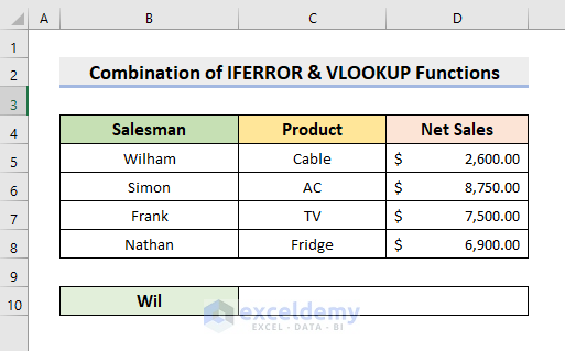
Method 2 – Combining the IFERROR & VLOOKUP Functions to Return Blank Instead of 0
The VLOOKUP function looks for a particular value in the specified range, and retrieves the corresponding value from another specified column if a match is found. Here, we’ll combine IFERROR & VLOOKUP functions to return a blank instead of 0.
In the following dataset, we’ll search for Wil in the range B5:D8. If a match is found, we’ll retrieve the value in the same row from the third column, otherwise we’ll return a blank cell.
Steps:
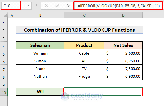
- Select cell C10.
- Insert the following formula:
=IFERROR(VLOOKUP(B10, B5:D8, 3,FALSE), "")- Press Enter.
A blank cell is returned as Wil is not in the range.
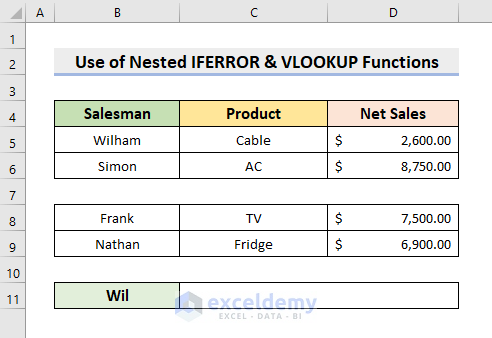
Method 3 – Using Nested IFERROR with the VLOOKUP Function to Return a Blank Instead of 0
In our last example, we’ll use multiple IFERROR and VLOOKUP functions to form a nested formula. In the below dataset, we’ll search for Wil in the range B5:D6 and B8:D9.
Steps:
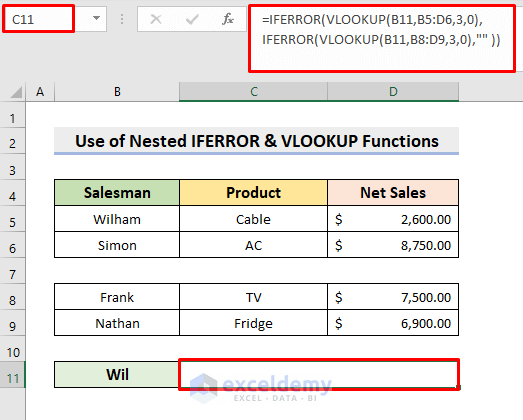
- Select cell C11.
- Enter the following formula:
=IFERROR(VLOOKUP(B11,B5:D6,3,0),IFERROR(VLOOKUP(B11,B8:D9,3,0),"" ))- Press Enter.
A blank cell is returned.
Read More: How to Use Multiple IFERROR Statements in Excel
Download Practice Workbook
Related Articles
- How to SUM with IFERROR in Excel
- How to Use IF and IFERROR Combined in Excel
- How to Use Conditional Formatting with IFERROR in Excel
<< Go Back to Excel IFERROR Function | Excel Functions | Learn Excel
Get FREE Advanced Excel Exercises with Solutions!
