Today I want to talk about one of the most important Excel functions – INDIRECT function.
Before doing that, I need to give you a brief introduction to the dollar sign ($) in the Excel formula.
You can’t understand INDIRECT function very well without a good knowledge of the dollar sign ($). You can skip to the next part if you are already familiar with the dollar sign ($).
Get an Idea How Absolute and Relative Reference Work
I’d like to explain it using an example.
Suppose you have a simple formula “=A1” in cell B1. This formula will change as “=A2” when you copy and paste it into cell B2.
If you paste it into cell C1, the formula will be “=B1”. And it will be “=B2” for cell C2.
Did you notice that both the column reference and row reference can change?
It is useful and allows a formula like SUM to be copied across or down the page and automatically refer to the new column or row.
But in some situations, you want some or all of the references to remain fixed when they are copied elsewhere and this is where the dollar sign ($) can be used.
The dollar sign ($) can precede the column reference, the row reference, or both.
Read More: Financial Planning with Excel Solver [2 Case Studies]
“A$1” means the row reference does not change when copied. “$A1” implies that column reference does not change while “$A$1” tells that both the column reference and row reference do not change when copied.
Here is a summary of what you will get if we change the above example a little bit. You can make a complicated formula and copy it elsewhere to see what will happen. It will help you better grasp relative reference and absolute reference.
| Cell B1 | Cell B2 | Cell C1 | Cell C2 |
| =A1 | =A2 | =B1 | =B2 |
| =A$1 | =A$1 | =B$1 | =B$1 |
| =$A1 | =$A1 | =$A1 | =$A2 |
| =$A$1 | =$A$1 | =$A$1 | =$A$1 |
Master Excel Formulas & Functions in Just 3.5 Hours!
with my FREE COURSE at Udemy.
Excel Formulas and Functions with Excel Formulas Cheat Sheet!
Let’s dig deep of Excel’s Indirect function
Indirect() function syntax and explanation
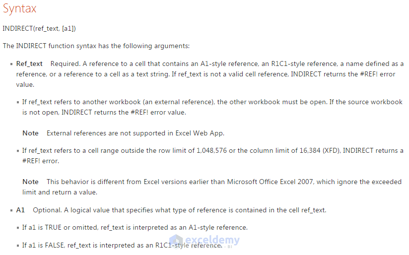
Excel’s INDIRECT function: Syntax [Click to enlarge]
In essence, it returns the references specified by a text string and the returned references can be immediately evaluated to display their content.
With the INDIRECT function, you can change the reference to a cell within a formula without changing the formula itself.
The below example can give you a better understanding of it.
The left section shows sample data and the right section applied the INDIRECT function to retrieve data from the left section.
I put formulas “=INDIRECT(A2) in cell D2, then copy and paste this formula down up to column D.
In order to give you a good explanation, I also put formulas as a text string for all cells (Cell D2, D3, D4 & D5) in column E.
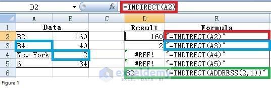
You can see that the content of cell A3 is “B4”, but the returned value is “2” instead of “B4” when I enter formula “=INDIRECT(A3)” in cell D3.
Why? What happened?
Because “B4” is a reference and Excel evaluated this reference and returns the content in cell B4 (see cells with blue borders).
Please note that if the reference is not valid, Excel will return “#REF!” error, just like what we get for cells D4 and D5. Obviously, “New York” and “6” are not valid references.
As for the reference, we all know that the ADDRESS function can yield the actual cell address associated with a row and column.
Then is it possible to use the INDIRECT function together with the ADDRESS function? What will you get?
Let’s take ADDRESS (2,1) as an example, Excel ADDRESS function will return “$A$2”.
In cell D6, entering the formula “=INDIRECT (ADDRESS (2,1))”, I get “B2” which is the content of cell A2.
The INDIRECT does not evaluate reference “B2”. Interesting?
You can compare this formula together with the formula in cell D2 to have a better understanding.
With the above knowledge, I will give you examples showing how to solve problems in real life.
Case 1: Change cell or range reference without changing the formula![]()
Suppose that we have data for the sales of 7 products in four regions (East, West, North, and South).
How can you use the INDIRECT function to calculate the total sales of any combination of consecutively numbered products, such as Product 1 through Product 4, Product 3 through Product 5, and so on?
Usually, we will use the formula “=SUM(D6:D9)” to compute the total sale of Product 1 through Product 4 in East and “=Sum(D8:D10)” to compute the total sale of Product 1 through Product 4 in East.
You can see that we need to modify the formula every time we want to see total sales of different products in one region. Obviously changing the formula is time-consuming if there are many regions.
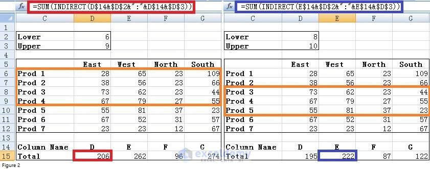
Figure 2
Luckily, we have another approach with the INDIRECT function.
Look at cell D15 in the above figure, the formula is “=SUM(INDIRECT(D$14&$D$2&”:”&D$14&$D$3))”.
Every cell reference within the INDIRECT part of this formula is evaluated to equal the contents of the cell.
D$14 is evaluated as D, $D$2 is evaluated as 6, and $D$3 is evaluated as 9. With the ampersand (&) included as the concatenation symbol, Excel evaluates this formula as “SUM(D6:D9)”, which is exactly what we want.
From the right section, you can see that by changing values in Cells D2 and D3, the formula in D15 is evaluated by Excel to be “SUM(D8:D10)” which is also what want.
Thus, by placing the starting and ending rows of the summation in cells D2 and D3 and using the INDIRECT function, all we need to do is to change the starting and ending row reference in D2 and D3 when we want to compute sales for a different combination of products.
The last point that needs your attention in figure 2 is the difference and similarities between the two formulas. The formula in cell E15 is just copied from cell D15. By copying and pasting, you don’t need to do manual work. But you have to make sure that what you get is right. That’s the reason why I mention dollar sign ($) at the beginning.
Case 2: Consolidate multiple worksheets into one master worksheet![]()
Suppose you have a workbook contains each employee’s hours of work and employee rating for January-May and you want to set up a master sheet that enables you to report all employee’s working hours or all employee’s overall rating for all months.
What will you do?
Since a figure can only include limited information. I only created a sample workbook with two source worksheets and one master worksheet (see below in Figure 3).
By only changing values in cell D2 in the master worksheet, you can see from the figure that we can choose to report all employee’s working hours or their overall rating. And the Excel will list the name of the report in cell B2.
How did I get this?
I entered formula “=INDIRECT(C$4&”!”&$D$2&$A5)” in cell C5, then copied and pasted into other cells in range C5:D11. “C$4” will be evaluated as “Lucy”.
By concatenating with “!”, we got the spreadsheet name “Lucy!”. “$D$2” was evaluated as “C” and “$A5” was evaluated as 3.
Altogether, the final reference evaluated by Excel is “Lucy!C3” and you can see from the lower-left part of the below figure that the content is 40. And 40 is just what we want.
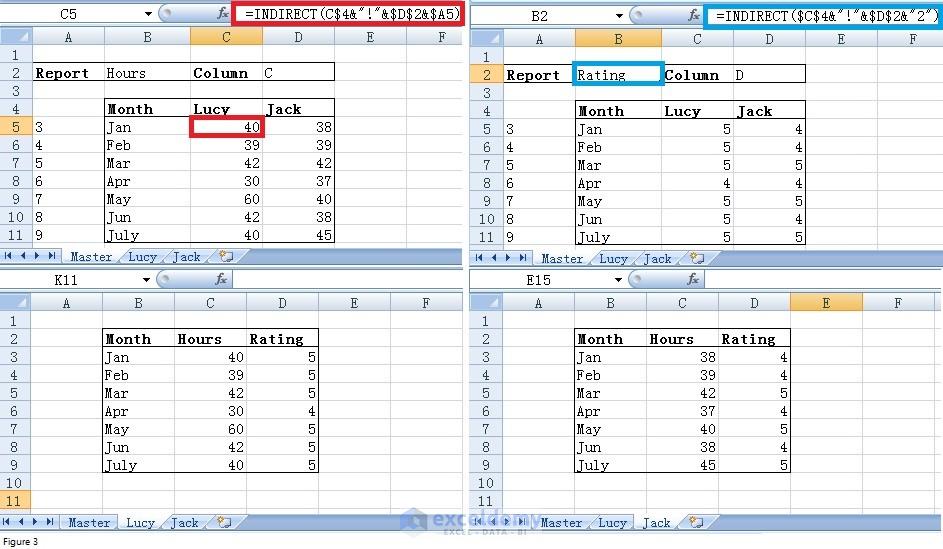
Figure 3
Since I did not place a dollar sign ($) between “$A” and “5” in the above formula, the formula will change to be “=INDIRECT(C$4&”!”&$D$2&$A6)” when it was copied into cell C6.
This is very important. Otherwise, you will 40 instead of 39. Obviously, 40 is not what we want.
Therefore, please remind that you should be very careful about the dollar sign ($).
Let’s move on to the next formula – “=INDIRECT($C$4&”!”&$D$2&“2”)” (upper left part of Figure 3).
Again, C$4&”!”&$D$2 will be evaluated as “Lucy!C” and by concatenating with 2, we get “Lucy!C2” and the content in that cell is “Hours”.
Since the second row is the same for all source worksheets – Lucy and Jack in our case, I decided to retrieve data only from the second spreadsheet and I placed a dollar sign (in red) before “C”.
You can compare the two formulas to see the differences and similarities.
With this workbook, you can add any number of rows into each source worksheet and any number of source worksheets.
As long as you fill the name of the added worksheet in the 4th row and put the reference number in column A, the master worksheet will give you all the final complete report.
Case 3: Combination of DIRECT with VLOOKUP to re-organize or retrieve data![]()
Sometimes we need to transpose vertical data into horizontal data, just as shown in Figure 4.
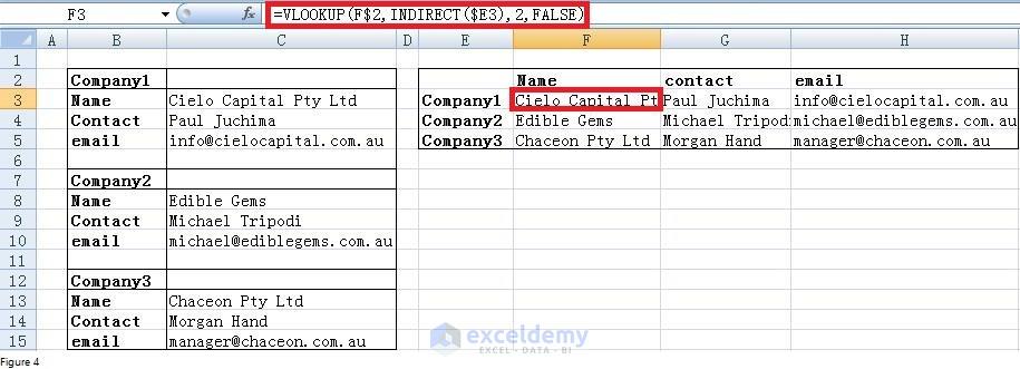
Figure 4
And in this kind of situation, the VLOOKUP function is often used. It is well known that the second argument for the VLOOKUP function should be the cell range that is to be searched for the first argument.
Then how can we combine the VLOOKUP function with the INDIRECT function? From the below figure, we can see that formula in cell F2 is “=VLOOKUP (F$2, INDIRECT($E3),2,FALSE)”.
The content of “$E3” is “Company1” and this is absolutely not a valid reference per our introduction at the beginning.
Then why Excel did not give “#ref!”? There must be something special.
Yes, you are correct. ”Company1” is the name for range B3:B5 in this case and that’s the reason why Excel did not return an error and how we combine VLOOKUP and INDIRECT. Therefore before entering
Therefore before entering the formula, we need to give all three ranges (B3:C5, B8:C10, and B13:C15) a name as “Company1”, “Company2”, and “Company3”, respectively.
To name a range can be done by following the below steps: Select the range of cells that contain the data we want to give a name; Right-click with the select range and click Name a Range or Define Name; Type the name for the range in the New Name dialog box; Click Ok.
This approach can also be used to search ranges from different worksheets then put the retrieved data in a master worksheet. You can figure out how to do this based on case 2 and case 3 in this post. This is a good exercise for you to test if have the master INDIRECT function or not.
Download working files
Download the working file from the link below.
Related Articles
- INDIRECT Function Excel: Get values from different sheet
- Excel Data Validation Based on Another Cell
- Excel Dynamic Range Based on Cell Value
- Excel Reference Cell in Another Sheet Dynamically


The Named Ranges in Case 3 should be B3:C5, B8:C10 and B13:C15.
Nice article!!!
Hi Jack. Thanks for pointing it out. I did not realize that I made a typo mistake.
Jack, I have notified it to the writer. She will answer soon 🙂