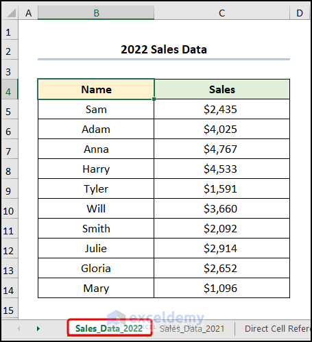
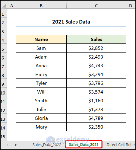
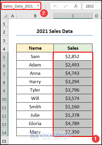
The two sample datasets show data on 2020 Sales shown in the B4:C14 cells which depict the Names of the sales reps and their Sales in USD respectively, and the 2021 Sales Dataset is shown in the following worksheet.
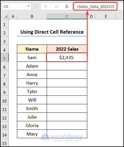
Method 1 – Using Direct Cell Reference
Steps:
- Select cell C5.
- Enter the below formula.
=Sales_Data_2022!C5
Here, “Sales_Data_2022!” is the name of the worksheet being referenced, while the C5 cell indicates the Sales value for Sam.
- Use the Fill Handle Tool to copy the formula into the cells below.
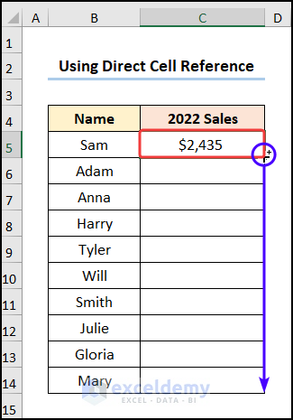
- Repeat the process in the following column.
=Sales_Data_2021!C5
Here, “Sales_Data_2021!” is the name of the worksheet being referenced, while the C5 cell indicates the Sales value for Sam.
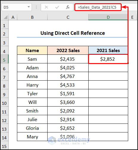
The resulting table should look like the image below.

Read More: How to Use OFFSET for Cell Reference in Excel
Method 2 – Utilizing INDIRECT Function
Steps:
- Select the C5 cell.
- Enter the below formula.
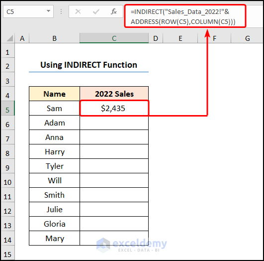
=INDIRECT("Sales_Data_2022!"&ADDRESS(ROW(C5),COLUMN(C5)))
Here, “Sales_Data_2022!” is the name of the worksheet being referenced, while the C5 cell indicates the Sales value for Sam.
- Select cell D5 to enter the 2021 Sales Data with the below formula.
=INDIRECT("Sales_Data_2021!"&ADDRESS(ROW(C5),COLUMN(C5)))
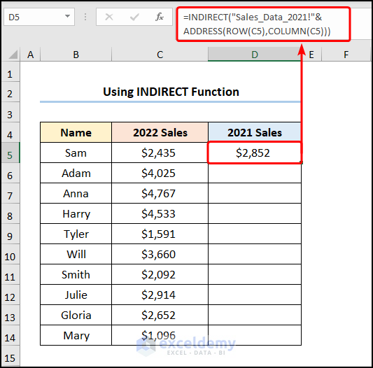
The results should look like the picture shown below.

Read More: How to Use Cell Value as Worksheet Name in Formula Reference in Excel
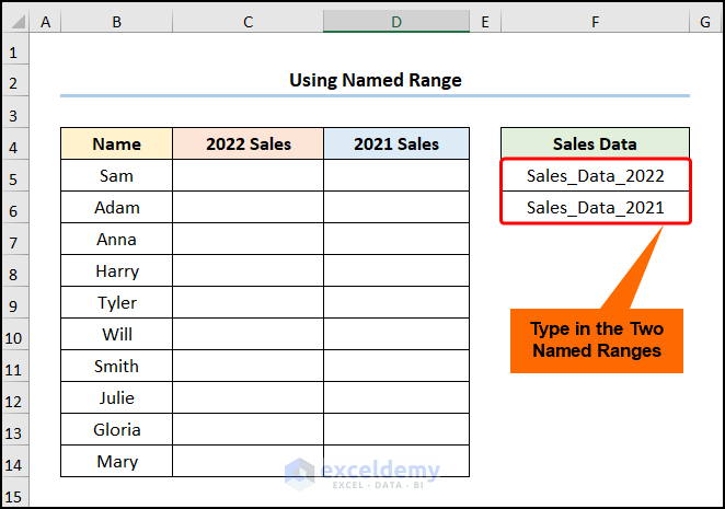
Method 3 – Combining Named Range and INDIRECT Function
Steps:
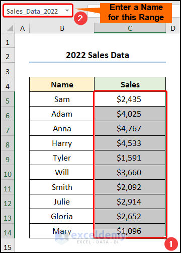
- Go to the Sales_Data_2022 worksheet.
- Select the C5:C14 cells.
- Enter a suitable name, in this case, Sales_Data_2022, in the Name Box.
- Give the C5:C14 range of cells the name Sales_Data_2021 in the Sales_Data_2021 worksheet.
- Enter the Named Ranges in the F5 and F6 cells as shown below.
Note: Please make sure to type in the exact names, otherwise you may get an error. If you’re having trouble with the exact names, you can bring up the list of Named Ranges by pressing the F3 key on the keyboard.
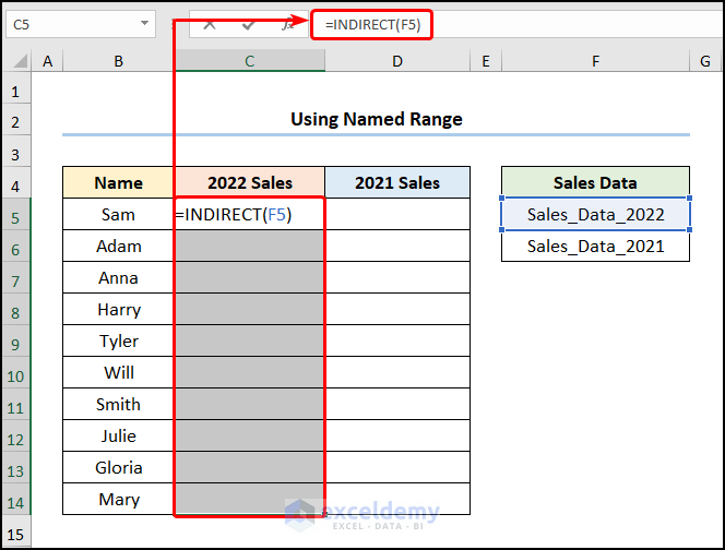
- Select the C5:C14 cells and paste the following formula.
=INDIRECT(F5)
The F5 cell represents the Sales_Data_2022 Named Range.
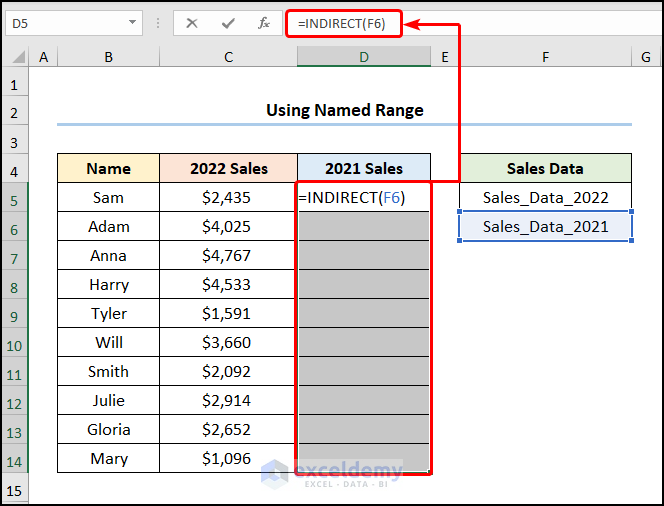
- Repeat the procedure for the D5:D14 cells.
=INDIRECT(F6)
The F6 cells refer to the Sales_Data_2021 Named Range.
The results should look like the screenshot below.
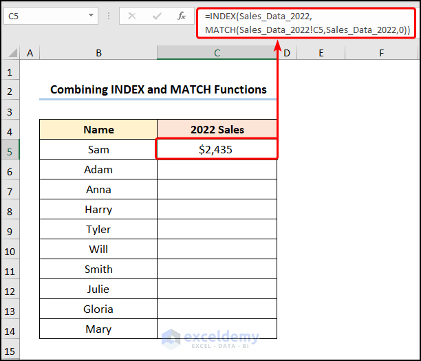
Method 4 – Employing INDEX and MATCH Functions
Steps:
- Go to the C5 cell and paste the following formula.
=INDEX(Sales_Data_2022,MATCH(Sales_Data_2022!C5,Sales_Data_2022,0))
Here the “Sales_Data_2022” refers to the Named Range and the C5 cell indicates the Sales value for Sam.
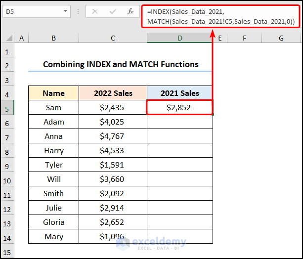
- Select the D5 cell and enter the formula below.
=INDEX(Sales_Data_2021,MATCH(Sales_Data_2021!C5,Sales_Data_2021,0))
Here the “Sales_Data_2021” refers to the Named Range and the C5 cell indicates the Sales value for Sam.
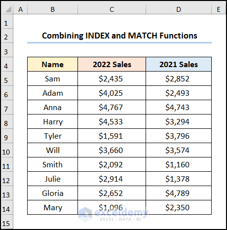
The results should appear as below.
Read More: How to Reference Cell by Row and Column Number in Excel
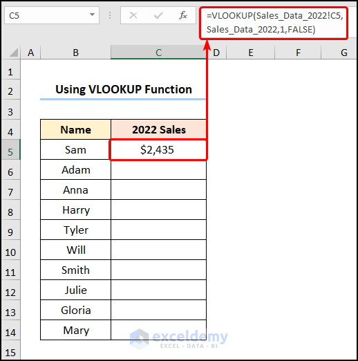
Method 5 – Applying VLOOKUP Function
Steps:
- Go to the C5 cell and paste the following formula.
=VLOOKUP(Sales_Data_2022!C5,Sales_Data_2022,1,FALSE)
Here, the “Sales_Data_2022!” represents the worksheet name, Sales_Data_2022 points to the Named Range, and the C5 cell indicates the Sales value for Sam.
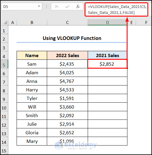
- Repeat the process in the D5 cell to insert the data for the year 2021.
=VLOOKUP(Sales_Data_2021!C5,Sales_Data_2021,1,FALSE)
“Sales_Data_2021!” refers to the worksheet name, the Sales_Data_2021 indicates the Named Range, and the C5 cell represents the Sales value for Sam.
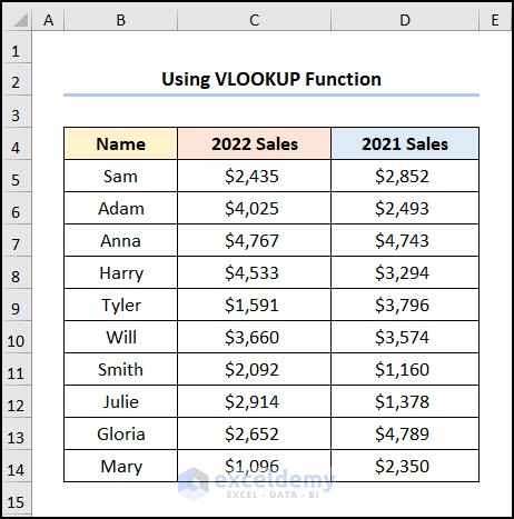
The results should appear as below.
How to Reference Cell in Another Sheet Based on Cell Value in Excel
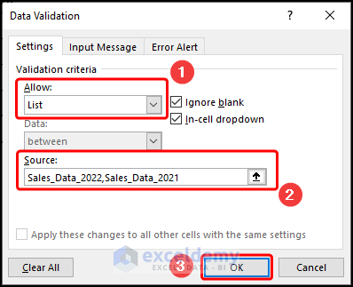
Steps:
- Go to the C7 cell.
- Navigate to the Data tab.
- Click on the Data Validation drop-down. This opens the Data Validation window.
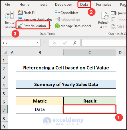
- In the Allow field, choose the List option.
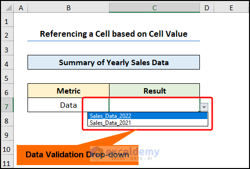
- In the Source field, enter the Named Ranges as defined in method 3.
This will insert a Data Validation drop-down in the C7 cell as shown in the image below.
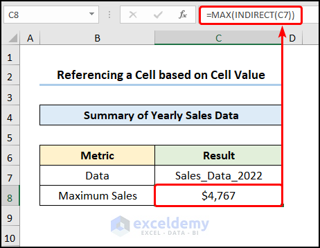
- Go to the C8 cell.
- Enter the below formula.
=MAX(INDIRECT(C7))
The INDIRECT function stores and returns the values of the Named Range to the current worksheet while the C7 cell refers to the Sales_Data_2022.
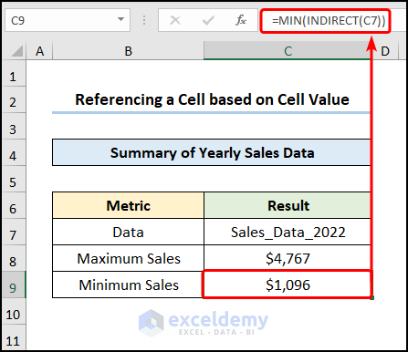
- Calculate the Minimum Sales value in the C9 cell with the MIN function below.
=MIN(INDIRECT(C7))
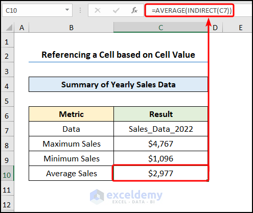
- Calculate the Average Sales by using the AVERAGE function as shown below.
=AVERAGE(INDIRECT(C7))
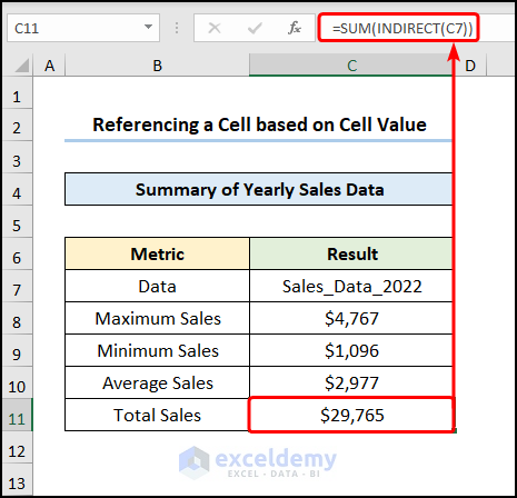
- Calculate the total sales in USD with the SUM function.
=SUM(INDIRECT(C7))
The results should look like the below image.
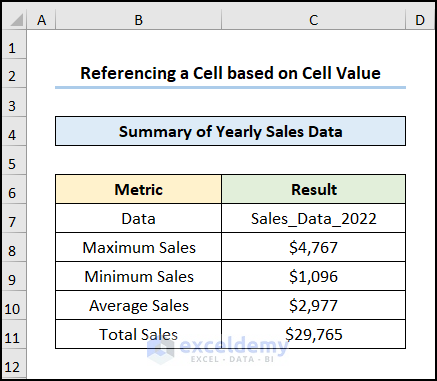
If you select Sales_Data_2021 from the drop-down then the results will appear from that sheet.

Read More: How to Reference a Cell from a Different Worksheet in Excel
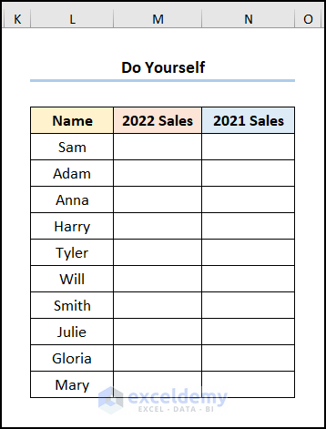
Practice Section
Download Practice Workbook
You can download the practice workbook from the link below.
Related Articles
- How to Display Text from Another Cell in Excel
- How to Reference Text in Another Cell in Excel
- How to Use Variable Row Number as Cell Reference in Excel
- Excel VBA Examples with Cell Reference by Row and Column Number
- Excel VBA: Cell Reference in Another Sheet
<< Go Back to Reference to Another Sheet | Cell Reference in Excel | Excel Formulas | Learn Excel
Get FREE Advanced Excel Exercises with Solutions!

These methods depend on the sheet name. Is there a method where the sheet name is dynamic? I want to reference cells from a sheet to the left of the current sheet, but the sheet name will change as the formula is carried through the entire workbook. Is there a formula for that? My workplace has VBA locked down, so that’s not an option.
Hello, DJ!
Thank you for your query.
To analyze your problem, I would say it would be impossible to automate the sheet names completely without saving the file as an xlsm file.
As far as I understood you want to create as many sheets as you want and then extract values from them in other sheets automatically whenever you want. In this regard, you want to address the sheets automatically without writing their names in the formulas.
Now, In this process, VBA codes are the most appropriate to use. Without VBA codes, you have another way to do this by using the GET.WORKBOOK() function. But, you will need to save the file as an xlsm file even in this process. But, as your VBA is locked down, I am afraid you would not be able to work with xlsm file.
So, I would say this would be quite impossible to solve your problem with VBA locked down.
Regards,
Tanjim Reza